
The most useful U.S. evidence for assessing UBI's supply chain impact is not a theory about automation. It is a spending ledger. In the OpenResearch unconditional cash study, 1,000 participants ages 21 to 40 in Texas and Illinois received $1,000 per month for three years; compared with the control group, recipients spent an average of $310 more per month, with the largest reported increases in food at $67, rent at $52, and transportation at $50 [1].
That pattern does not behave like a clean, economy-wide demand injection. It behaves like a mix shift. If a national UBI ever moved from proposal to policy, the first planning question would not be whether “consumer demand” rises. It would be where the new spend lands, which networks touch those categories, and whether the receiving supply chains have enough capacity to absorb the load without turning the cash transfer into longer lead times, tighter bookings, or higher prices.

The First Signal Is Essential-Category Uplift
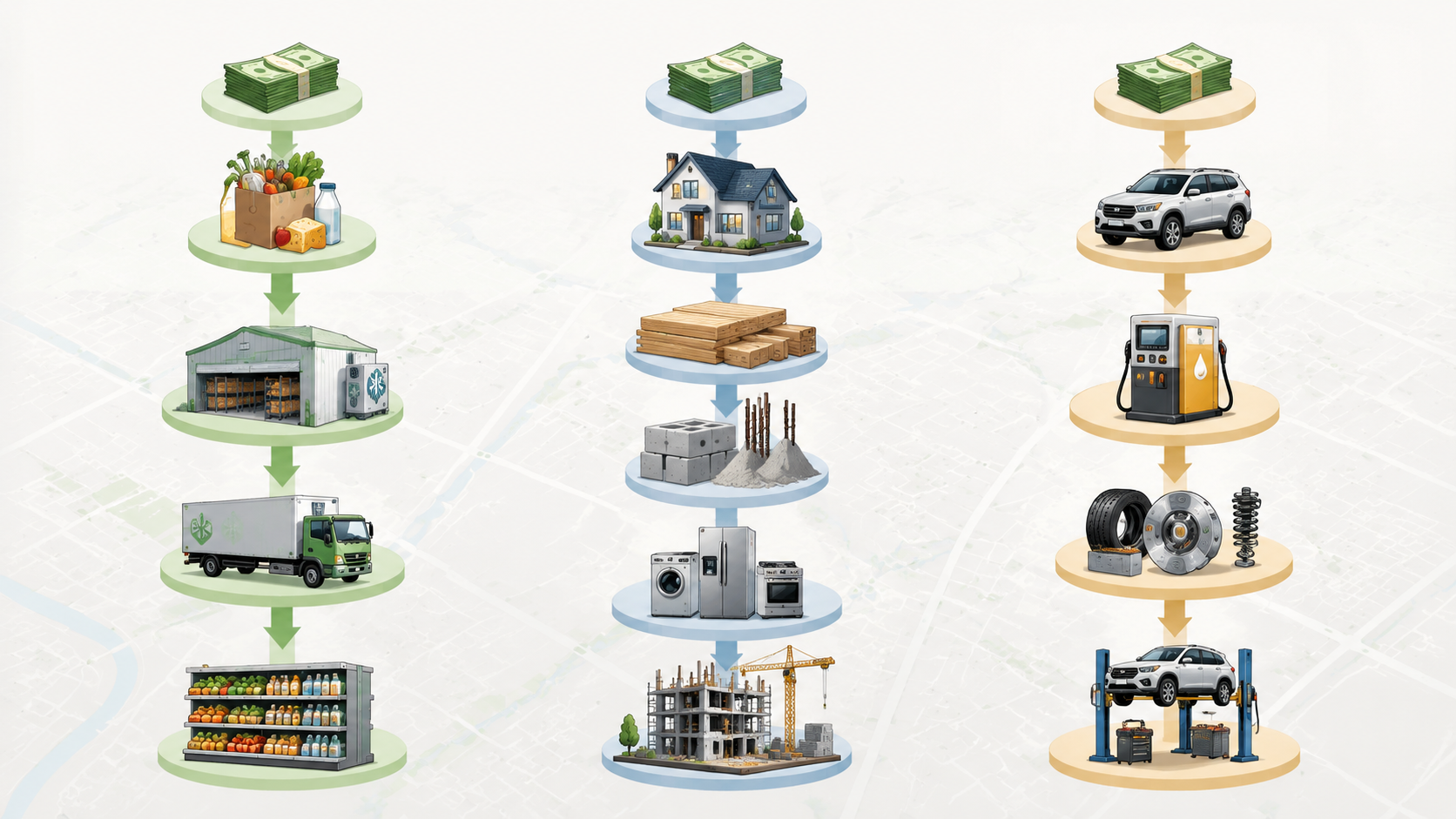
For a demand team, the OpenResearch breakdown is more actionable than a headline about poverty reduction or economic stimulus because the categories map to operating decisions. Food touches grocery replenishment, refrigerated transport, regional DC throughput, packaging, and last-mile availability. Rent points toward housing demand and the supply chains attached to housing formation, repair, turnover, fixtures, and appliances. Transportation spend touches fuel, maintenance, parts, vehicle access, and mobility services.
| OpenResearch spending category | Monthly increase | Supply chain functions most exposed |
|---|---|---|
| Food | +$67 | Grocery replenishment, cold chain, temperature-controlled warehousing, last-mile grocery delivery |
| Rent | +$52 | Housing turnover, residential materials, fixtures, appliances, repair and maintenance supply |
| Transportation | +$50 | Fuel distribution, auto parts, maintenance networks, vehicle access and mobility services |
Those are first-order signals, not a national forecast. The study did not put every household in a city, state, or country on a guaranteed income. It measured the behavior of selected individuals in two states. That matters because a single recipient can increase grocery spend without changing the economics of a local grocery network; a saturated geography can change store traffic, labor scheduling, replenishment timing, supplier allocation, and upstream production plans.
Still, the category pattern is too concrete to ignore. A planner does not need national certainty to build a scenario layer. If a policy proposal has a plausible path to adoption, and the best available U.S. spending evidence points to food, rent, and transportation, those categories deserve earlier stress-testing than broad discretionary baskets.
Food Demand Would Hit Cold-Chain Capacity First
Food is the cleanest operational signal in the study. A $67 monthly increase does not tell a grocery operator which SKUs move, but it does say the first UBI scenario should not start with luxury durables. It should start with baskets that move through grocery, mass retail, dollar stores, club channels, foodservice-adjacent retail, and local delivery networks [1].
The planning consequence is not simply “ship more food.” Food demand is constrained by perishability, delivery cadence, shelf life, labor availability, and cold-storage positioning. A modest category uplift can be harder to serve than a larger uplift in a slow-moving durable category because the execution window is shorter. If the increase concentrates in fresh food, frozen food, dairy, meat, or prepared meals, the binding constraint may be refrigerated trailer availability or store-level labor rather than supplier production.
This is where AI-enabled forecasting has a practical role. A model should not take “UBI adopted” as a single binary variable and smear the same adjustment across every category. It should separate essential categories, regions with lower baseline income, store formats, service levels, and known capacity pinch points. The same scenario logic used for route shocks or commodity disruptions can be repurposed for demand shocks; the difference is that the disruption begins in the household budget rather than at a port, border, or supplier site. Teams already building scenario libraries for logistics can treat UBI as another macro overlay, alongside the methods used in predictive analytics in logistics.
Rent Spend Is a Housing Signal, but Not a Simple Construction Forecast
The $52 increase in rent spending is easy to overstate. It does not prove that a UBI would immediately create a wave of new housing starts, nor does it identify how much of the increase went to moving, upgrading, staying current on rent, household formation, or absorbing higher rent levels. It does, however, mark housing as one of the first categories where extra cash showed up [1].
For supply chains tied to housing, that distinction matters. If the spending supports household stability, the demand effect may appear in maintenance, furnishings replacement, small appliances, utilities setup, repair parts, and local services. If it supports mobility or household formation, the signal may move closer to building materials, fixtures, appliances, flooring, paint, and last-mile delivery for bulky goods. If it mainly gets captured by rent inflation in constrained markets, the physical-goods uplift could be much smaller than the dollar increase suggests.
That is why rent should enter a forecast as a branching assumption, not as an automatic construction-materials multiplier. A national UBI scenario for a home improvement retailer, appliance manufacturer, or building-materials distributor should be segmented by housing supply conditions. Markets with vacant units, available labor, and active construction capacity can translate household cash into physical activity differently from markets where the next available unit is already scarce.
Transportation Spend Creates a Mobility Load, Not Just an Auto-Sales Story
The transportation increase in OpenResearch was $50 per month, close to the rent increase and below the food increase [1]. It is enough to matter, but too general to turn into a vehicle-sales forecast. Transportation spend can mean fuel, insurance, repairs, public transit, rideshare, vehicle payments, parts, or the ability to accept work farther from home.
The most defensible supply chain interpretation is a wider mobility load. Auto parts networks would watch maintenance demand. Fuel and convenience channels would watch trip frequency and local driving patterns. Service centers would watch labor scheduling and parts availability. Retailers would watch whether better mobility changes store access, delivery preferences, and pickup behavior. The effect may sit partly inside transportation supply chains and partly inside every retail network that depends on whether a customer can reach a store or job.
The Cash Did Not All Become Immediate Consumption
One reason UBI should not be modeled as a uniform demand surge is that recipients did not spend the full transfer. OpenResearch reported that bank savings grew 25%, and spending on others, including gifts, loans, and charity, rose 26% [1]. Scott Santens’ review of the study emphasizes the same point: looking only at immediate personal consumption misses where cash can move next, including savings, household resilience, and transfers to other people [2].
For planners, savings are not irrelevant simply because they do not show up in next month’s POS data. Savings can delay demand, smooth demand, or change the timing of larger purchases. Spending on others can also move demand away from the original recipient’s basket and into another household’s needs. A forecasting team that treats the full transfer as near-term retail demand will overstate the immediate load. A team that ignores the transfer because not all of it was spent will miss the category reweighting that did occur.
Individual Pilots Do Not Show Saturation Effects
The OpenResearch study is the right place to start, but it is not the right place to stop. A national UBI would not distribute cash to isolated individuals inside otherwise unchanged communities. It would change the purchasing power of whole regions at the same time, which means local demand, supplier response, labor markets, and capacity utilization would all move together.
Alaska’s Permanent Fund Dividend is one reason planners should keep saturation effects separate from individual effects. The dividend has operated since 1982, and the evidence base around it is often used as a real-world analogue for broad cash distribution rather than a small pilot. In the research summarized for UBI spending debates, Alaska is associated with a 17% increase in part-time employment through local demand stimulus, a signal that economy-wide effects can appear outside the original recipient basket [2].
Kenya’s saturation UBI evidence points to a different planning lesson: demand increases do not automatically create measurable inflation if the local economy has slack capacity. The relevant supply chain question is not simply whether households receive more money. It is whether suppliers, carriers, warehouses, stores, service providers, and labor pools can respond without hitting a constraint. Santens’ inflation framework makes that point directly by treating capacity, competition, supply-side policy, and downstream savings as variables that shape whether cash transfers become price pressure [3].
Those analogues should not be imported as if Alaska, Kenya, and a hypothetical U.S. national UBI are interchangeable. They are useful because they prevent a planning team from overfitting to one U.S. individual-level study. They say, in different ways, that the same cash transfer can produce different operating outcomes depending on saturation, slack capacity, competitive response, and local constraints.
Where the Forecast Overlay Belongs
A national UBI scenario does not belong unexamined in baseline demand. Baseline implies the business has enough evidence that the pattern is already embedded or highly probable. The U.S. has not run a national UBI, so the better treatment is a scenario family: a set of named overlays that can be switched on, compared, and stress-tested against category capacity.
| Planning layer | How UBI should be represented | Why it matters |
|---|---|---|
| Baseline forecast | Do not load national UBI as baseline unless policy is enacted and early data confirms the pattern | Prevents a speculative macro assumption from contaminating normal demand history |
| Macro overlay | Apply category-weighted uplift to food, rent-linked, and transportation-related demand | Uses the strongest first-order evidence without pretending SKU-level certainty |
| Scenario layer | Create separate versions by funding mechanism, capacity slack, and regional exposure | Shows whether the same policy becomes growth, bottleneck, inflation pressure, or reallocation |
| Promotional adjustment | Keep separate from UBI unless offers specifically interact with household cash timing | Avoids confusing policy-driven income effects with retailer-created demand |
This is a natural fit for AI scenario planning because the policy variable is too large to leave in a spreadsheet note and too uncertain to hard-code into one forecast. A planning system can hold multiple UBI cases at once: an essential-category uplift case, a tax-funded compression case, a constrained-capacity case, and a high-slack absorption case. The value is not that the model knows the future. The value is that the model forces the team to state which mechanism it is testing.
Teams that already model geopolitical route shocks or commodity shocks have a useful template. A UBI scenario can be built with the same discipline used in AI scenario planning for Middle East commodity and route shocks or broader AI supply chain resilience planning: define the shock, map the exposed nodes, set the transmission mechanism, and decide which metrics would confirm or reject the case.
Funding Mechanism Is the Discretionary-Goods Question
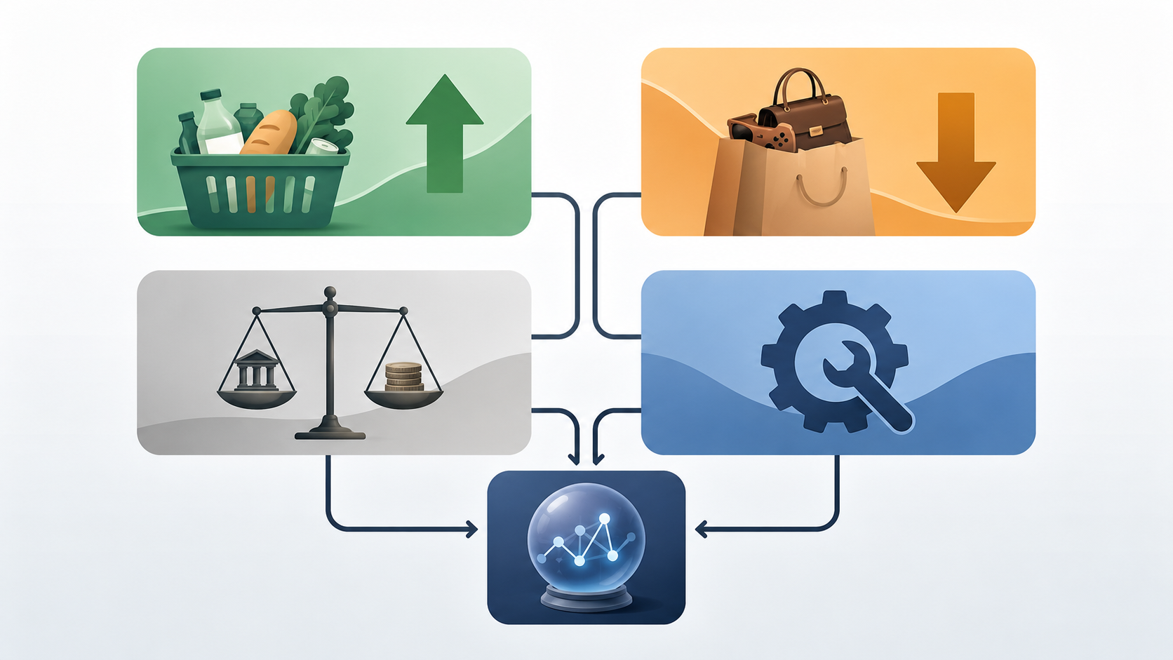
Discretionary compression is plausible, but it should not be asserted without the funding side. If a UBI is deficit-financed, tax-financed, funded through consumption taxes, funded through payroll changes, or paired with benefit consolidation, the demand compression lands in different places. A consumption-tax-heavy design would pressure price-sensitive discretionary categories differently from a funding design aimed at high-income households or corporate income.
That is where many UBI supply chain discussions get sloppy. They add demand to essential goods from the payment, then vaguely subtract demand from discretionary goods because “someone has to pay for it.” A planning model needs the second half translated into a mechanism. Which consumers lose disposable income? Which categories see effective prices rise? Which suppliers face higher labor or tax costs? Which imported goods become more exposed than domestic services? Without that bridge, discretionary compression is a guess with a policy label attached.
The cleanest model structure is to keep direct spending and funding effects separate. Direct spending uses the OpenResearch evidence: food, rent, and transportation receive the first overlay. Funding effects sit in a separate scenario branch and can reduce demand in non-essential goods, raise supply chain costs, or both. The net forecast is the combination, not the starting assumption.
What to Monitor Before Policy Becomes Reality
A demand team does not have to wait for a signed national UBI bill to prepare. It can define the indicators that would move a scenario from watchlist to active planning. The useful signals are not generic election headlines. They are variables that change item-location forecasts, lane plans, cold-storage bookings, supplier commitments, and labor assumptions.
- Payment design: monthly amount, eligibility, household treatment, timing, and whether payments are universal or targeted.
- Funding design: consumption tax, payroll tax, income tax, deficit financing, benefit replacement, or mixed structure.
- Category sensitivity: food, rent-linked goods and services, transportation, and other essentials with high exposure to lower-income household cash flow.
- Capacity slack: cold storage utilization, carrier availability, housing supply, service labor, supplier lead times, and regional warehouse throughput.
- Confirmation data: early POS movement, basket composition, rent and mobility indicators, savings behavior, and transfer timing effects.
Food-sector teams can go one level deeper because the OpenResearch signal is strongest there. A grocery demand model should test whether uplift appears in staples, fresh categories, prepared foods, private label, or delivery-heavy baskets. That is the same forecasting discipline used when evaluating localized demand signals for new menu items or grocery assortments, as in AI demand forecasting for food-related launches. The category is supported by evidence; the SKU path still has to be learned.
The Capacity Test Decides Whether Demand Becomes Growth or Friction
The same dollar of additional demand can produce four different operating outcomes. It can become real volume growth if supply is elastic. It can become a bottleneck if warehousing, labor, or transport is tight. It can become inflation pressure if sellers have pricing power and limited capacity. Or it can become reallocation if households shift spend from one category to another while total physical volume changes less than expected.
That capacity test is the bridge between UBI evidence and supply chain action. OpenResearch tells planners where the first spending signal appeared. Alaska and Kenya-style analogues warn that saturation and slack capacity change the outcome. Inflation frameworks add the variables that decide whether the receiving network can absorb the shock [1][2][3].
For procurement teams, that means UBI should not only sit in a demand forecast. It should also appear in commodity and supplier-risk scenarios. If food demand rises in a constrained environment, packaging, refrigerated capacity, agricultural inputs, and regional labor costs can become part of the same planning case. The same logic applies to housing-linked materials and transportation parts. Procurement groups using AI commodity price forecasting would need to tag UBI not as a political topic, but as a possible demand-side driver in selected categories.
A Usable UBI Planning Frame
The practical forecast frame is narrow, which is what makes it useful. First, apply an essential-category uplift scenario anchored in the OpenResearch spending categories. Second, keep savings and spending-on-others as timing and redistribution variables, not as vanished demand. Third, run saturation and capacity cases separately from individual-recipient behavior. Fourth, model discretionary compression only through a specified funding mechanism.
Under that frame, a national UBI would likely reweight demand toward essential-good supply chains based on the best available U.S. spending evidence. Food, housing-linked demand, and transportation deserve the first stress tests. Discretionary goods may compress, but the magnitude and location depend on how the program is paid for. Capacity determines whether the new demand becomes volume growth, bottlenecks, inflation pressure, or a quieter reallocation across household budgets.
References
- Unconditional Cash Study, OpenResearch
- Did Sam Altman's Basic Income Experiment Succeed or Fail UBI?, Scott Santens
- 17 Key Variables That Determine UBI's Inflationary Impact, Scott Santens
Comments
Join the discussion with an anonymous comment.