
A static ETA usually fails quietly before it fails visibly. The transportation manager sees one clean arrival time in the TMS; the dispatcher sees a driver who has slowed down; the warehouse sees a dock slot that may or may not hold; customer service sees a customer who will ask for an answer before the next carrier milestone arrives. By the time the ETA is obviously wrong, the useful decision window may already be gone.
That is the real question behind predictive ETA in logistics: not whether a system can produce a better-looking timestamp, but whether it can keep recomputing when the route stops behaving like the plan. Carrier-provided ETAs are reported as 40–60% inaccurate beyond three days out when they lack visibility into port congestion, weather routing, and cascading delays.[1] In one vendor comparison, standard routing API ETAs averaged a 16-hour mean error when predicted 24 hours in advance, while ML-based ETAs reached roughly 2-hour mean absolute error on the same horizon.[2]
Those figures are useful, but only with their labels attached. A 24-hour-ahead ocean or freight estimate is not the same problem as a last-mile stop prediction inside a dense urban delivery network. A vendor-reported benchmark is not an industry baseline. A 15-minute window is not comparable with a 9-hour air freight accuracy band. ETA accuracy without horizon, mode, and tolerance window is not a metric; it is decoration.
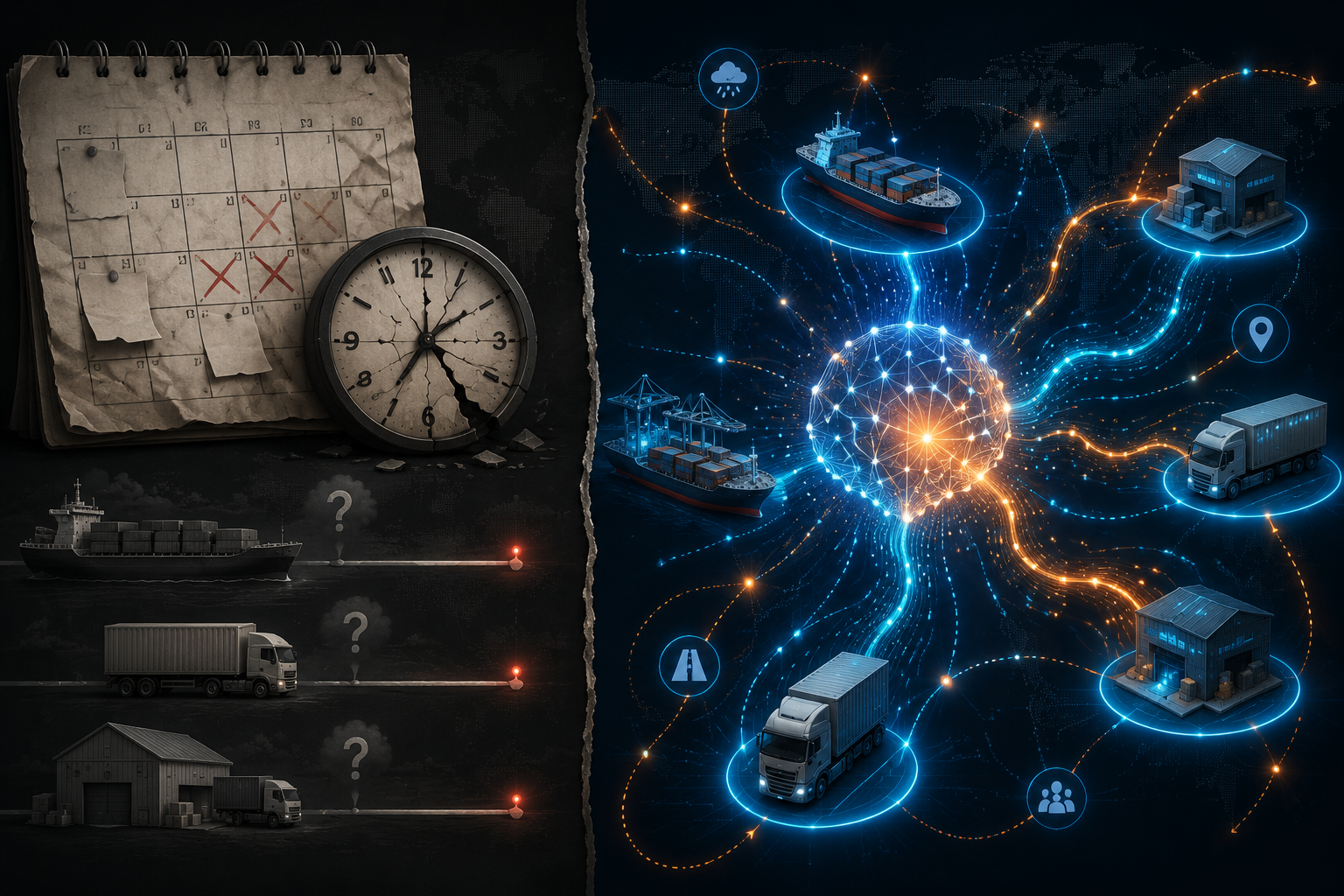
The shift is architectural, not cosmetic
The old ETA stack starts with a plan: scheduled departure, route distance, service time assumptions, carrier milestones, and maybe a traffic estimate. When the plan is still a reasonable proxy for the shipment, that can be enough. The trouble begins when the shipment becomes part of a living network: a vessel waits outside a congested port, a driver extends a break, rain changes traffic speed, a warehouse falls behind, or a missed appointment pushes a downstream route into a different time-of-day pattern.
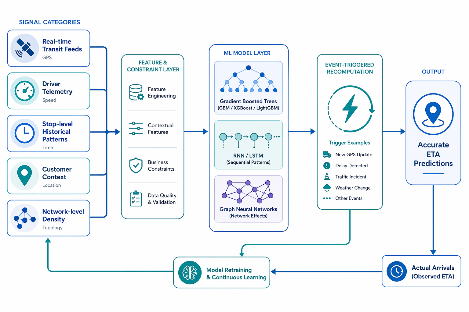
Production-grade predictive ETA treats arrival time as a continuously revised inference over a changing data graph. Signals enter, features are recalculated, constraints are applied, the model predicts for a specific mode and horizon, and new events trigger another pass. The model matters, but the data architecture is the product. A clever algorithm on stale milestones is still a stale ETA.
That is why strong last-mile claims deserve both attention and restraint. Locus reports 95%+ accuracy within 15-minute windows for last-mile ETA use cases and describes predictive systems processing 180+ variables compared with rule-based systems handling 10–20 constraints in batch runs.[3] That kind of tolerance window can change dock labor, customer notifications, and route intervention decisions. It should not be casually transferred to ocean, air, or long-haul freight without checking the signal density and prediction horizon.
What the system has to see before it can predict
A predictive ETA system needs a wider surface area than many visibility dashboards expose. The minimum useful signal set spans real-time transit feeds, driver or vehicle telemetry, stop-level historical patterns, customer and delivery context, and network-level delivery density.[3][4] Leave out one category, and the model may still return a timestamp, but the operating team should know which kind of failure it is now blind to.
| Signal category | What it contributes | What breaks when it is missing |
|---|---|---|
| Real-time transit feeds | Current location, milestone movement, route progress | The system keeps trusting the plan after the shipment has drifted |
| Driver or vehicle telemetry | Speed, dwell, breaks, driving behavior, vehicle-level movement | ETA misses the difference between distance remaining and progress actually being made |
| Stop-level history | Service time, dwell patterns, appointment behavior, time-of-day effects | The model treats every stop as average even when the location is predictably slow |
| Customer and delivery context | Delivery windows, priority, receiver constraints, access conditions | The ETA may be mathematically plausible but operationally unusable |
| Network-level density | How nearby routes, facilities, lanes, and nodes are behaving | The model underestimates cascading delay and local congestion effects |
The important word here is not "more." It is coverage. Two hundred parameters are not automatically better than fifty; a long feature list can hide duplicate, delayed, or low-quality fields. But broad parameter coverage matters when each parameter closes a real operational blind spot: the difference between scheduled and actual departure, historical dwell at that consignee, traffic speed on the next leg, carrier reliability on that lane, weather along the corridor, or the density of other deliveries competing for the same local capacity.
The same is true for the 180+ variable contrast. Constraint depth is useful when it reflects the things that can actually invalidate an ETA: appointment windows, driver hours, service times, vehicle type, stop sequence, road restrictions, port dwell, warehouse capacity, customer availability, and downstream commitments. A rule-based batch run can encode some of these constraints, but it tends to ask, "What did we think was true when the plan ran?" Predictive ETA has to ask, "What is true enough right now to change the decision?"
Data quality work sits underneath all of this. If vehicle pings arrive late, carrier milestones are inconsistent, stop IDs are not normalized, or actual arrival timestamps are captured differently by region, the model will learn from noise. Teams building this capability usually need the same discipline described in a supply chain AI data quality checklist: freshness, completeness, lineage, standard definitions, and exception handling before the model ever gets praised or blamed.
From signals to an ETA someone can act on
The workflow is less mysterious than the phrase "AI-powered ETA" suggests, but it is less forgiving than a demo screen suggests.
- Ingest live and historical signals from transit feeds, telematics, stops, customers, and the surrounding network.
- Normalize those signals into shipment, route, stop, facility, carrier, and time-window entities.
- Convert raw fields into features and constraints the model can use.
- Predict against a defined mode, horizon, and tolerance window.
- Trigger recomputation when meaningful events arrive.
- Feed actual arrivals, misses, and exception outcomes back into retraining.
The normalization layer is where many ETA programs either become usable or stay fragile. A truckload, an ocean container, and a last-mile stop do not share the same event grammar. "Arrived" may mean gate arrival, yard arrival, dock check-in, proof-of-delivery timestamp, or carrier-reported milestone. If those events are not reconciled, model evaluation becomes a debate about timestamps rather than accuracy.
Feature engineering then turns logistics behavior into model-readable evidence. A raw GPS ping becomes current speed, distance remaining, dwell duration, and deviation from expected route progress. A stop history becomes expected service time by location, day, time window, and delivery profile. A carrier history becomes reliability on a lane or at a node. A network signal becomes congestion or delay pressure around ports, facilities, roads, or delivery clusters.
The prediction itself should always be framed. "ETA is 10:20" is not enough. The useful version is closer to: for this last-mile stop, with current telemetry and stop history, the model predicts arrival between 10:15 and 10:30; or for this ocean-linked inland move, 24 hours out, the expected error is measured in hours rather than minutes. The tolerance window determines whether the answer can support a customer notification, dock reslot, labor hold, expediting decision, or only broad exception monitoring.
Recomputation is where predictive ETA earns its name
Batch ETA can be adequate when the network is quiet and decisions are slow. Freight and delivery networks are often neither. Event-driven predictive ETA recomputes when a new signal changes the probability of arrival: a traffic jam, a port closure, a driver break extension, a missed departure, a dwell event that exceeds normal duration, or a downstream stop that becomes infeasible. Estuary and Shippeo both describe predictive ETA as requiring live feeds and event-driven processing rather than batch-only updates.[5][6]
The timing of that recomputation matters as much as the math. If an exception arrives after the warehouse has already released labor, or after customer service has already promised a delivery window, the ETA may be accurate and still useless. Good systems are tuned around decision latency: how soon the signal arrives, how quickly the prediction changes, and whether the revised ETA reaches the control tower, TMS, WMS, customer notification layer, or dispatcher workflow before someone has to act.
This is also where predictive ETA becomes an integration problem. A control tower that displays a recalculated ETA but does not change exception queues, appointment workflows, or notification rules is only halfway connected. For teams evaluating that operating layer, the practical question is similar to the one behind AI-powered supply chain control towers: does the prediction change the work, or does it just decorate the screen?
Which models fit which ETA failures
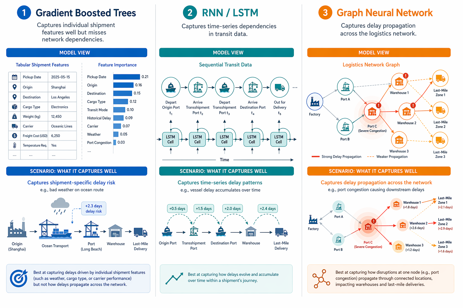
Model choice should follow the failure pattern. A logistics ETA problem with clean tabular shipment attributes is not the same as one dominated by time-series behavior or network delay propagation. The useful comparison is not which model family sounds most advanced; it is which source of error the model can actually reduce.
Gradient boosted trees: strong on structured shipment features
Gradient boosted trees are a natural fit when the system has rich tabular data: lane, carrier, origin, destination, appointment type, stop count, historical dwell, distance remaining, day of week, time of day, weather category, and current delay against plan. They are often practical because logistics data is full of structured fields that are messy but not inherently sequential.
Their weakness is not that they are old-fashioned. It is that a per-shipment feature table can flatten the living sequence of a trip. If the difference between an on-time and late arrival depends on how delay accumulated over the last several events, or how congestion is propagating through a network, boosted trees may need help from time-aware or graph-aware features.
RNN and LSTM models: useful when the path matters over time
RNN and LSTM approaches are designed for sequential dependencies. In ETA work, that means they can learn from the order and timing of events: departure, slow progress, dwell, recovery, another delay, then arrival. This is closer to how dispatchers read a shipment. They do not only ask where the asset is; they ask how it has been moving and whether the latest behavior resembles previous late or recovered trips.
The tradeoff is operational. Sequential models need consistent event streams. If telematics is intermittent, carrier milestones arrive in bursts, or event definitions vary by partner, the model can learn artifacts of reporting behavior instead of transportation behavior. That does not make the approach wrong; it raises the bar for ingestion and event standardization.
Graph neural networks: promising where delay propagates
Graph approaches deserve attention because many ETA errors are not isolated shipment errors. A delayed vessel affects containers, drayage appointments, warehouse capacity, outbound truck schedules, and eventually customer delivery windows. Kumo and project44 both frame predicted ETA in terms of networked supply chain conditions, including congestion, weather, carrier behavior, and cascading disruption.[1][7]
A graph neural network can represent ports, facilities, lanes, vehicles, shipments, and stops as connected nodes and edges. That lets the model learn how delay pressure moves through the network instead of treating each shipment as independent. Conceptually, that is exactly the pattern many independent ETA models miss: port congestion plus weather plus carrier history may produce a delay larger than any one feature implies.
The caution is evidence. The conceptual case for graph models is strong where delay propagation matters, but broad production evidence is thinner than the architectural argument. For many enterprises, the first gating issue will not be whether a graph model is theoretically superior. It will be whether their shipment, facility, carrier, route, and event data can support a reliable graph in the first place.
Accuracy benchmarks need their denominator
ETA benchmarks are easy to overuse because the numbers are tempting. The responsible comparison keeps five labels visible: prediction horizon, transport mode, tolerance band, data inputs, and source type.
| Benchmark | What it measures | How to read it |
|---|---|---|
| 40–60% inaccurate beyond three days | Carrier-provided ETAs beyond a three-day horizon | A warning about long-horizon visibility gaps, not a universal failure rate |
| 16-hour mean error vs. roughly 2-hour MAE | Routing API compared with ML-based ETA at a 24-hour horizon | A vendor comparison showing a large architecture gap, not an industry average |
| 95%+ within 15-minute windows | Vendor-reported last-mile predictive ETA accuracy | Highly relevant for dense last-mile decisions; not transferable without matching conditions |
| 9-hour accuracy | Air freight tracking benchmark | A reminder that mode-specific ceilings differ sharply |
The air freight example is useful precisely because it refuses the fantasy of one universal ETA target. FourKites describes a 9-hour accuracy benchmark for air freight tracking, a very different tolerance environment from 15-minute last-mile delivery windows.[8] Air shipments involve different handoffs, milestone availability, and operational decisions. A nine-hour band may be too coarse for a delivery appointment and still meaningful for upstream exception management in air freight.
Academic work adds methodological seriousness, but it should not be inflated into broad deployment proof. TU Berlin and Kpler present work on forecasting inland vessel ETA with predictive analytics, while the ScienceDirect research cited in this area reflects constrained research settings rather than enterprise-wide production coverage.[9][10] That kind of work is valuable for model design and evaluation discipline. It does not remove the need to test performance on a company's own lanes, carriers, geographies, and event quality.
The feedback loop separates a predictor from a reporting tool
Actual arrivals are not just outcomes; they are training data. A predictive ETA system that captures actual arrival times, compares them with predicted windows, tags the miss, and feeds the result into retraining can improve in ways a static rule set cannot. AWS demonstrates this basic learning loop in a shipment ETA example using SageMaker Canvas, where historical shipment data supports ETA prediction and subsequent model use.[11]
The hard part is deciding what the system should learn from. If a shipment arrived late because the driver ignored the planned sequence, that is different from a carrier capacity issue, a receiver delay, a weather event, or a bad original appointment time. If the actual-arrival timestamp is captured at proof of delivery in one region and gate arrival in another, retraining may reward the wrong behavior. Feedback loops compound accuracy only when the labels are trustworthy.
This is where enterprise architecture and operating process meet. The model needs miss reasons, exception codes, arrival definitions, and retraining cadence. The operations team needs to know when the model has changed enough to affect escalation rules. If agents or automated workflows will act on predictive ETA, the governance bar rises again; the same broader questions around agentic AI in procurement and logistics workflows apply once an ETA starts triggering work rather than merely informing it.
How to evaluate readiness
The cleanest vendor demo is still the wrong starting point. Start with the decisions the ETA must support. A customer notification may need a narrow, stable window. A dock reslot may need confidence before a labor cutoff. A long-haul exception queue may tolerate a wider band if it catches risk early enough. A control tower may need fewer false positives more than it needs another decimal point of accuracy.
- Define the mode, horizon, and tolerance window before comparing accuracy claims.
- Audit whether live signals cover transit movement, telemetry, stop history, delivery context, and network density.
- Check recomputation triggers and latency, not just model output frequency.
- Validate actual-arrival definitions and feedback data before trusting retraining.
- Test by lane, carrier, geography, facility type, and decision use case instead of accepting one blended accuracy score.
A predictive ETA program is ready when its accuracy is measured in the same units as the decision it is meant to improve. If the warehouse needs a 15-minute arrival window and the system can only provide a two-hour band, it may still be useful for exception monitoring but not for labor scheduling. If the carrier milestone feed is hours late, a sophisticated model may still miss the dispatcher’s intervention window. If actual arrivals are poorly labeled, retraining can make the system more confident without making it more correct.
This also keeps ROI claims grounded. Predictive ETA can support measurable value when it reduces avoidable calls, missed appointments, idle labor, expedites, or customer uncertainty. But that value depends on whether the prediction enters the workflow in time to change an action. Teams that need the financial layer can evaluate it alongside other use cases in supply chain AI ROI analysis, after they know what the ETA can reliably support.
Predictive ETA works when it has enough live signal breadth, constraint depth, training history, and event-driven recomputation to support the decision being made. That is a narrower claim than "AI fixes ETA," and a much more useful one.
References
- ETA Prediction, Kumo, link
- Machine Learning: Fixing the ETA Problem in Logistics, SeaVantage, link
- Engineering Predictive ETA Accuracy Guide for Last Mile, Locus, link
- Predictive ETA Freight, FleetWorks, link
- Predictive Freight ETA Machine Learning, Estuary, link
- Improving ETA Predictions in Transport: Challenges and Solutions, Shippeo, link
- What Is Predicted Estimated Time of Arrival in Supply Chain?, project44, link
- Data Science Breakthrough in Air Freight Tracking, FourKites, link
- Case Study: Forecasting Inland Vessel ETA with Predictive Analytics, Kpler, link
- ScienceDirect article S2352146524001716, ScienceDirect, link
- Predict shipment ETA with no-code machine learning using Amazon SageMaker Canvas, AWS, link
Comments
Join the discussion with an anonymous comment.