
How Traditional Demand Forecasting Works and Where It Breaks
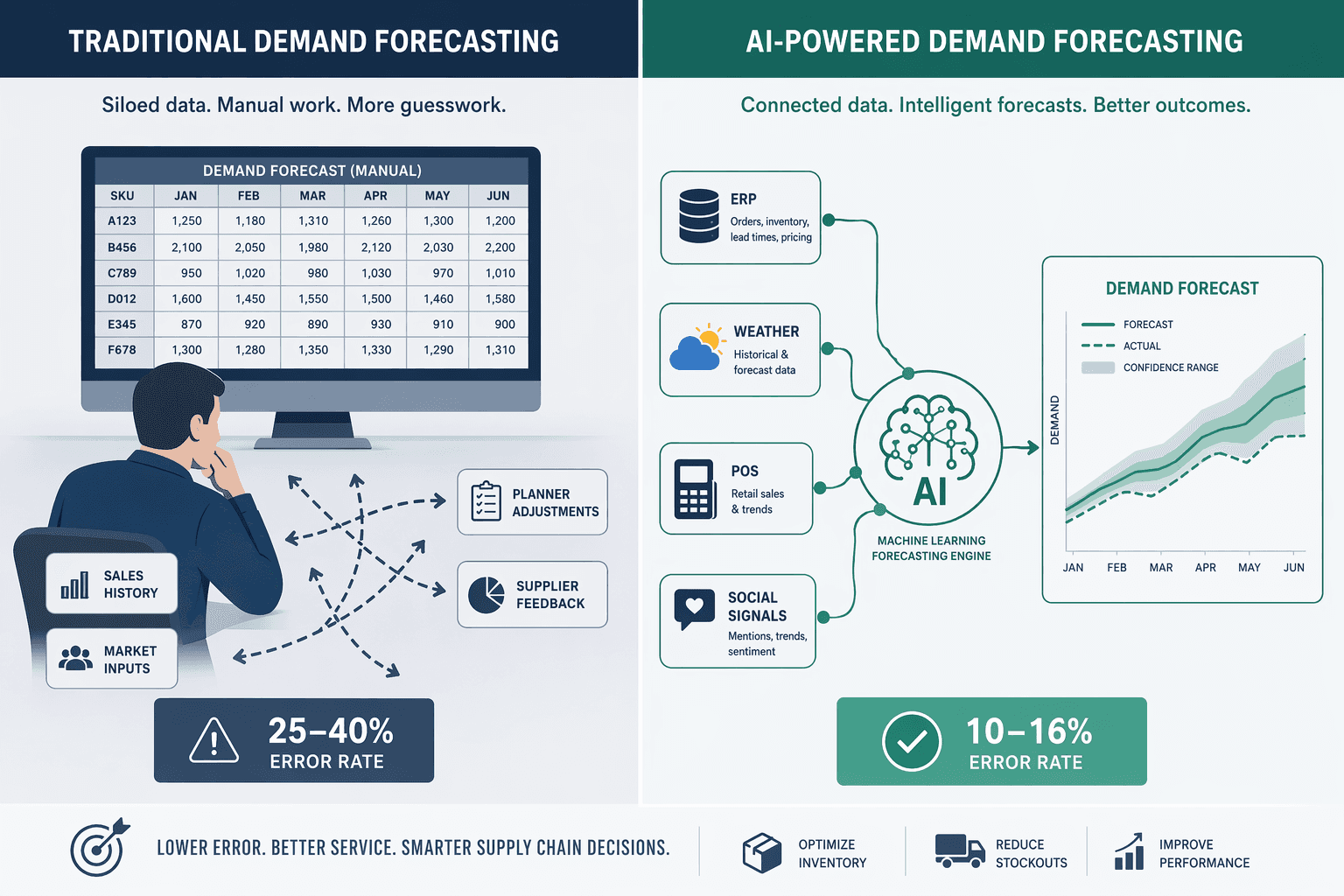
Most supply chain organizations running traditional demand forecasting rely on a small set of statistical methods: moving averages, exponential smoothing, and ARIMA (AutoRegressive Integrated Moving Average) models. These techniques were developed in the mid-20th century and were designed for a world where demand patterns were relatively stable, data was scarce, and computing power was expensive. They work by identifying historical trends and seasonality, then projecting those patterns forward.
The fundamental limitation is that these models are static. Once a traditional model is trained on historical data, its parameters remain fixed until a planner manually intervenes to recalibrate it. In practice, many organizations update their statistical models quarterly or even annually. During the intervals between updates, the model is blind to shifts in consumer behavior, competitor actions, supply disruptions, or macroeconomic changes.
Traditional methods also operate in a data silo. They typically ingest only internal historical sales volumes and perhaps a basic calendar of promotions and holidays. They cannot incorporate external signals — weather patterns, social media sentiment, web traffic, port congestion data, or real-time point-of-sale (POS) feeds — that increasingly drive demand in modern markets. This limitation becomes critical in volatile environments: a traditional model cannot distinguish between a genuine demand signal and noise from a one-time event.
The consequences are measurable. According to data cited by GroupBWT and the IJSAT 2025 study, traditional forecasting methods report error rates of 25–40%. In industries with high SKU complexity or seasonal volatility — apparel, consumer electronics, fresh food — error rates at the upper end of that range are common. A forecast that is wrong by 30–40% is not a forecast; it is a guess that forces planners to compensate with safety stock, expedited freight, and manual overrides.
- Static parameters: Models do not adapt between manual recalibration cycles, typically quarterly or annually.
- Limited data scope: Only internal historical sales and basic calendar inputs; no external or real-time data.
- Lagging indicators: Traditional methods detect shifts only after they appear in historical data, making them reactive.
- Linear assumptions: ARIMA and exponential smoothing assume linear relationships that break down in volatile markets.
- High error rates: 25–40% forecast error is typical, forcing costly buffers in inventory and capacity.
How AI-Driven Forecasting Differs: Continuous Learning and Multivariate Analysis
AI-driven demand forecasting represents a fundamentally different approach to the problem. Instead of fitting a static equation to historical data, machine learning models are trained to detect complex, non-linear patterns across hundreds or thousands of variables simultaneously. The core technical differences are not incremental improvements on traditional methods — they are architectural shifts in how forecasts are generated, validated, and updated.
The first difference is continuous model retraining. AI models can be retrained daily or weekly as new data arrives, meaning the forecast adapts to the most recent demand signals rather than waiting for a quarterly recalibration. This is particularly valuable in fast-moving categories where consumer preferences shift rapidly. A model that learned demand patterns from last year's holiday season can be updated with this week's POS data to reflect current buying behavior.
The second difference is multivariate data ingestion. AI systems can consume data from sources that traditional methods cannot handle: real-time POS transactions, weather forecasts, social media trends, web traffic, competitor pricing changes, economic indicators, and even satellite imagery of retail parking lots. As Oracle notes in its overview of AI demand forecasting, these systems incorporate data on historical sales, sales pipelines, consumer behavior, demographics, competitor activity, seasonal and market trends, weather events, holiday schedules, economic conditions, website traffic, and social media engagement. The ability to process this breadth of inputs is what allows AI models to detect demand signals before they appear in historical sales data.
The third difference is probabilistic output. Traditional methods produce a single point forecast — "we will sell 10,000 units next month" — with no indication of the range of possible outcomes. AI models can generate probabilistic forecasts that express demand as a distribution: "there is an 80% probability that demand will fall between 8,500 and 11,500 units." This probabilistic view is far more useful for inventory decisions, safety stock calculations, and risk assessment because it quantifies uncertainty rather than hiding it.
Real-world deployments across industries demonstrate these capabilities in practice. The AI Demand Forecasting in Production article on ChainSignal documents how companies in retail, CPG, pharmaceuticals, and other verticals have applied these techniques to specific operational problems — from seasonal assortment planning to promotional lift prediction.
- Continuous retraining: Models update daily or weekly, not quarterly, adapting to the latest demand signals.
- Multivariate inputs: Ingest POS, weather, social media, economic data, and other external signals alongside internal sales history.
- Probabilistic forecasts: Output demand distributions with confidence intervals rather than single point estimates.
- Non-linear pattern detection: Identify complex relationships and interactions that linear models cannot capture.
- Automated feature engineering: ML models can discover which variables are predictive without manual specification.
Head-to-Head Accuracy Benchmarks: Traditional vs. AI
The most frequently cited question from supply chain executives evaluating AI forecasting is straightforward: how much more accurate is it? The answer depends on industry, product mix, data maturity, and market volatility, but the available research provides a consistent range that is useful for building a business case.
The table below compiles the key accuracy benchmarks from multiple sources. These figures should be treated as ranges rather than guarantees — actual results vary by deployment context.
| Metric | Traditional Methods | AI / ML Methods | Source |
|---|---|---|---|
| Forecast accuracy (point estimate) | 60–75% | 85–95% | OnePint.ai |
| Forecast error rate (MAPE / WAPE) | 25–40% | 10–16% | IJSAT 2025 (via GroupBWT) |
| Error reduction vs. baseline | — | 20–50% | McKinsey (via IBM, Oracle, GroupBWT) |
| Stockout-related lost sales reduction | — | Up to 65% | McKinsey (via GroupBWT, SR Analytics) |
| Inventory cost reduction | — | 20–35% | SR Analytics |
| Weighted Absolute Percentage Error (WAPE) reduction | — | 40–75% | GroupBWT |
| Forecast bias reduction | — | 30–70% | GroupBWT |
The AWS whitepaper on demand forecasting provides a more conservative but still significant benchmark: organizations that implemented ML forecasting improved accuracy by 10–20%, which translated into a 5% reduction in inventory costs and a 2–3% increase in revenue. While these figures are from an earlier generation of ML capabilities, they are useful as a lower-bound estimate for organizations with less mature data environments.
The variation across these sources underscores an important point: accuracy improvement is not a fixed number. Companies with clean, granular data (three to five years of SKU-level transaction data, as Invisible Tech notes) and stable demand patterns will see improvements at the lower end of the range. Companies operating in volatile markets with rich external data sources — and the infrastructure to integrate them — can achieve the higher end.
The ROI Realization Timeline: What Returns to Expect and When
One of the most common misconceptions about AI demand forecasting is that ROI materializes immediately after deployment. In practice, returns follow a phased timeline that depends on data integration, model maturity, and organizational adoption. Understanding this timeline is critical for setting executive expectations and securing continued investment through the early phases.
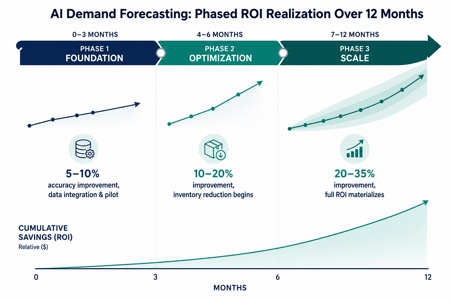
SR Analytics provides a phased ROI framework based on retail implementations, which aligns with patterns observed across multiple industries. The timeline below reflects typical outcomes for organizations with reasonably clean data and dedicated implementation teams.
| Phase | Timeframe | Forecast Accuracy Improvement | Primary Activities |
|---|---|---|---|
| Phase 1: Foundation | Months 1–3 | 5–10% | Data integration, baseline model training, pilot on 1–2 product categories |
| Phase 2: Optimization | Months 4–6 | 10–20% | Model tuning, additional data sources added, inventory reduction begins |
| Phase 3: Scale | Months 7–12 | 20–35% | Full category rollout, S&OP integration, secondary benefits materialize |
The 5–10% improvement in months 1–3 may seem modest, but it is important context: during this phase, the team is typically still cleaning data, establishing integration pipelines, and running the AI model in parallel with the existing forecasting process. The model is learning from historical data and being validated against actual outcomes. Organizations that skip this validation phase and push directly to full deployment often encounter model drift and trust issues with planning teams.
By months 4–6, the model has accumulated enough training cycles to begin outperforming the traditional baseline consistently. This is when inventory reduction starts to appear on the balance sheet. SR Analytics reports that AI reduces inventory costs by 20–35% at this stage, and McKinsey's research shows up to 65% fewer lost sales from stockouts.
The 20–35% accuracy improvement by month 12 represents the point at which the model has been retrained across multiple seasonal cycles and has learned to incorporate external data sources. At this stage, the secondary benefits — reduced manual override labor, faster S&OP cycles, improved supplier negotiations — begin to compound the direct forecasting ROI.
Decision Framework: Which Product Categories Need Which Approach
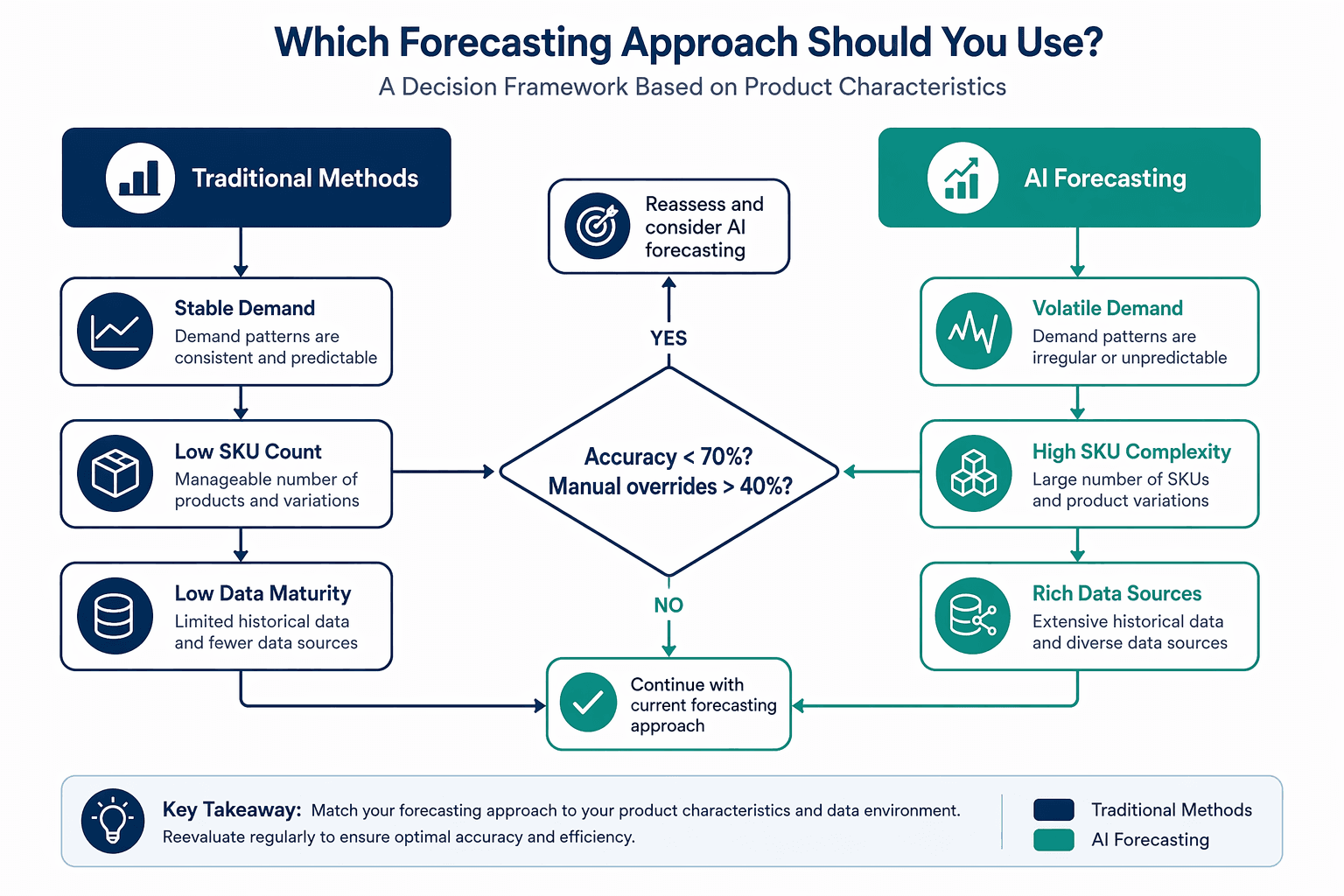
Not every product category needs AI forecasting. In fact, applying AI to stable, low-volume categories with clean historical patterns can be over-engineering that adds complexity without proportional benefit. The decision of which approach to use should be driven by product characteristics, data availability, and the cost of forecast error.
The decision framework below routes product categories based on three primary dimensions: demand volatility, SKU complexity, and data maturity. The central trigger question — "Is forecast accuracy below 70%? Are manual overrides exceeding 40%?" — serves as a practical heuristic for identifying categories where traditional methods are failing.
| Product Characteristic | Traditional Methods Suitable | AI Methods Recommended |
|---|---|---|
| Demand pattern | Stable, low variance, predictable seasonality | Volatile, trend-shifting, promotional spikes |
| SKU count per category | Low (under 100 SKUs) | High (hundreds or thousands of SKUs) |
| Data history available | 2+ years of clean, consistent data | 3–5 years of SKU-level data with external signals |
| External data relevance | Minimal (no weather, social, or economic impact) | Significant (weather, promotions, competitor activity) |
| Cost of forecast error | Low (commodity, long lead times, substitutable) | High (perishable, seasonal, high-margin, custom) |
| Manual override rate | Under 20% of SKU-months | Over 40% of SKU-months |
For categories that fall into the "AI recommended" column, the next step is to assess data readiness. As Invisible Tech notes, three to five years of SKU-level transaction data is the practical standard for AI forecasting; less than two years, and the model is effectively guessing. Data quality — completeness, consistency, and the absence of uncorrected stockout periods — has a more direct impact on forecast accuracy than model selection itself.
Specific Triggers for Upgrading to AI Forecasting
Beyond the product-level decision framework, there are organization-wide signals that indicate it is time to move from traditional to AI-driven forecasting. These triggers are measurable, observable, and directly tied to operational and financial outcomes.
- Persistent forecast accuracy below 70%: If your weighted forecast accuracy has been below 70% for two or more consecutive quarters despite manual override efforts, the underlying model is not capturing the demand structure of your business.
- Manual override rates exceeding 40%: When planners are manually adjusting nearly half of all forecasts, the system has lost credibility. The labor cost of these overrides — and the inconsistency they introduce — is a hidden operational expense.
- Declining inventory turnover: If inventory turns are decreasing while forecast error remains flat, the organization is compensating for poor forecasts with additional safety stock. This is a direct working capital drain.
- Increasing stockout costs: Rising expedited freight costs, lost sales due to stockouts, or emergency production runs are symptoms of a forecasting system that cannot anticipate demand shifts quickly enough.
- Inability to incorporate external data: If your planning team cannot systematically include weather forecasts, promotional calendars, or economic indicators in the forecasting process, you are leaving predictive signals on the table.
- S&OP cycle time is constrained by forecasting: When the monthly S&OP process is delayed because planners are still debating forecast numbers, the forecasting system has become a bottleneck rather than an enabler.
For organizations that identify with three or more of these triggers, the business case for upgrading is strong. The next step is evaluating specific platforms. The 7 Best AI Demand Forecasting Tools for Enterprise in 2026 comparison on ChainSignal provides a structured capability assessment of the leading platforms, including methodology, integration requirements, and deployment models.
The Cost of Delay: How Much Not Upgrading Costs Per Quarter
The decision to delay an AI forecasting upgrade is not neutral — it carries a measurable quarterly cost that accumulates across multiple dimensions of the P&L. For organizations that meet the upgrade triggers described above, the cost of inaction can be quantified and presented alongside the investment required for the upgrade.
| Cost Category | Quarterly Impact (Estimate) | Source / Basis |
|---|---|---|
| Excess inventory carrying costs | 20–35% of current inventory holding costs | SR Analytics: AI reduces inventory costs by 20–35% |
| Lost revenue from stockouts | Up to 65% of stockout-related lost sales | McKinsey: AI reduces stockout lost sales by up to 65% |
| Markdowns from overstock | Variable, typically 10–30% of overstock value | Industry benchmark; varies by category and seasonality |
| Manual override labor | 10–20 hours per planner per week | IBM: Idaho Forest Group reduced forecasting time from 80+ hours to under 15 per cycle |
| Expedited freight premiums | 5–15% of total freight spend | Attributed to emergency replenishment from poor forecasts |
To put these figures in perspective, consider the McKinsey Global Institute estimate that generative AI could have a $60–110 billion annual impact in the pharmaceutical sector alone. While that estimate covers the full range of AI applications — not just demand forecasting — it illustrates the scale of value at stake when AI is applied to planning processes across an industry.
For a mid-market organization with $500 million in annual revenue and typical inventory carrying costs of 20–25%, a 20–35% reduction in inventory costs translates to $2–4 million in annual savings. Adding stockout reduction, markdown minimization, and labor savings, the total annual benefit often reaches 1–3% of revenue. The AI Use Cases in Supply Chain by Function article provides additional ROI benchmarks across procurement, warehouse operations, and logistics for broader context.
Implementation Path: From Pilot to Enterprise
The MIT maturity model for AI in supply chain planning provides a structured path from initial pilot to enterprise-wide adaptive forecasting. This framework, cited by GroupBWT, defines four stages with distinct investment levels, timelines, and capability milestones.
| Stage | Timeline | Investment Range | Key Milestones |
|---|---|---|---|
| Pilot | 0–3 months | $100K–$500K | Single category or region; parallel run with existing process; data pipeline validation |
| Expansion | 6–12 months | $500K–$2M | 3–5 categories or regions; model retraining automation; S&OP integration begins |
| Enterprise | 18–24 months | $2M–$10M | Full category rollout; external data integration; probabilistic forecasting in use |
| Adaptive | 36+ months | $10M+ | Continuous retraining; autonomous exception handling; full digital twin integration |
The pilot stage is the most critical. Organizations that rush this phase — skipping data quality validation, running the AI model without a parallel comparison to the existing process, or selecting a category that is too complex for a first attempt — often fail to build the trust needed to expand. The recommended approach is to select a product category that meets three criteria: high data quality (clean, complete SKU-level history of at least three years), moderate demand volatility (not the most stable category, but not the most chaotic), and a supportive category manager who is willing to be the internal champion.
Data readiness is the single most common failure point in the pilot phase. As Invisible Tech emphasizes, ERP integration is the most frequent technical bottleneck, and uncorrected stockout periods cause AI models to learn suppressed demand as genuine patterns. Organizations should budget 4–8 weeks for data assessment and pipeline construction before the model sees its first training cycle.
For readers beginning this journey, the Implementing AI Forecasting Without the Hype guide provides a detailed walkthrough of data readiness assessment, model selection criteria, and vendor evaluation. The How to Evaluate and Select AI-Powered Demand Forecasting Tools step-by-step guide covers the vendor selection process in depth, including RFI templates, proof-of-concept design, and evaluation scoring frameworks.
Comments
Join the discussion with an anonymous comment.