For supply chain leaders evaluating AI forecasting models, the first decision is not whether a model is “advanced.” It is whether the model can see the demand signals that actually move the business. If demand is mostly explained by each SKU’s own sales history, a statistical or tree-based model may be enough. If demand depends on substitutions, shared promotions, supplier constraints, product hierarchies, store clusters, or customer behavior spread across multiple tables, time-series-only forecasting starts to leave material information outside the model.
That is the practical reason to think in tiers. The useful taxonomy is not a ladder every company must climb. It is a way to decide which architecture deserves evaluation given the organization’s data environment: SKU history depth, SKU count, product interdependency, promotion intensity, and supplier complexity.

The decision starts with what the model is allowed to observe
AI demand forecasting generally combines historical demand with other variables to predict future demand more dynamically than manual planning or simple extrapolation, including signals such as seasonality, promotions, weather, and market changes.[1] That broad definition is helpful, but it hides a sharper architectural question: are those signals flattened into a single row per SKU-location-period, or can the model reason across relationships among products, stores, promotions, suppliers, and constraints?
Kumo.ai’s published analysis argues that time-series-only models can miss roughly 25–30% of demand signal because important relationships often live in separate relational tables rather than in the target sales history itself.[2] That figure should be treated as vendor-published analysis, not a universal law. Still, the underlying point is important for model selection: a forecast architecture that only sees one SKU-store history at a time cannot directly model many of the mechanisms planners already know matter.
Promotion is the clearest example. Kumo.ai reports that promotions drive 20–40% of retail volume, while many forecasting tools still reduce promotions to binary flags.[2] A binary flag can tell the model that an event occurred. It cannot, by itself, represent promotion type, depth, overlapping campaigns, substitution effects, supplier readiness, or whether a competing product was also discounted.

A five-tier taxonomy of AI forecasting models
The tiers below are best read as evaluation boundaries, not maturity labels. A lower-tier model can be the right choice when the business problem is narrow, the history is stable, and relational complexity is low. A higher-tier model can be wasteful when the required data does not exist or cannot be governed reliably.
| Tier | Model family | Best fit | Where it usually breaks |
|---|---|---|---|
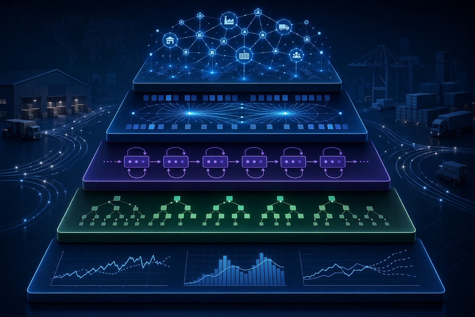
| 1 | Statistical baselines: ARIMA, Prophet, exponential smoothing | Long, clean history; stable seasonality; limited SKU interdependence; low promotion complexity | Weak handling of nonlinear external drivers and relationships among products, stores, and suppliers |
| 2 | Tree-based ensembles: XGBoost, LightGBM, random forests | Flat feature tables with calendar, price, inventory, event, and lag variables; many commercial forecasting deployments | Each SKU-location is commonly modeled as an isolated record, so cross-product and network effects are indirect |
| 3 | Recurrent deep learning: LSTM, GRU, DeepAR | Large sets of related time series where global patterns can transfer across SKUs or locations | Better temporal learning, but still limited when key drivers sit in complex relational structures |
| 4 | Transformer forecasting: Temporal Fusion Transformer, Informer, Autoformer, hybrid architectures | Longer dependencies, many covariates, and richer temporal context where compute cost is acceptable | Higher compute and storage requirements; architectural sophistication can exceed planning-data readiness |
| 5 | Graph neural networks and relational foundation models | Demand shaped by substitutions, complements, promotions, supplier constraints, product hierarchies, and multi-table enterprise data | Emerging category; strongest evidence is still concentrated in vendor benchmarks and technical publications |
Tier 1: statistical baselines
Statistical baselines remain useful because they are transparent, fast to run, and easy to challenge. They work best when a planner can explain most demand movement from the series itself: recurring seasonality, a stable trend, and enough history for the model to separate signal from noise.
Their limitation is not that they are old. It is that they see too little. A peer-reviewed IJSAT 2025 study cited by GroupBWT places traditional forecasting accuracy in a 25–40% MAPE range, a broad range that should not be interpreted as a benchmark for every category or company.[3] The more useful lesson is that baselines set a floor. If a more complex model cannot beat a well-built baseline on the planning metric that matters, the architecture is not earning its cost.
Tier 2: tree-based ensembles
Tree-based ensembles are often the commercial workhorse because they handle nonlinear features, missing values, categorical encodings, calendar effects, price changes, inventory positions, and engineered lags with relatively strong performance and manageable operational complexity. For many planning teams, this is where “AI forecasting” first becomes operational rather than experimental.
The ceiling appears when the data has been flattened too aggressively. If each SKU-store-week is represented as one row, the model can learn from features attached to that row. It does not naturally understand that one item substitutes for another, that a supplier delay affects a whole family of products, or that a promotion on one SKU changes the baseline of a neighboring SKU. Those relationships can be engineered, but the modeling burden shifts to feature design.
Tier 3: recurrent deep learning
Recurrent architectures such as LSTM, GRU, and DeepAR changed the evaluation question by allowing models to learn global patterns across many related series rather than training every item in isolation. Optimix Solutions describes DeepAR’s advantage as the ability to transfer patterns from similar items, including zero-shot prediction for new products with no sales history.[4]
That matters in assortments with frequent launches, sparse histories, or long-tail SKUs. A new item can borrow information from items with similar behavior. But the gain still depends on whether the model receives the right similarity signals. If product relationships are only implicit, or if launch context is stored outside the training table, the recurrent model may be learning from an incomplete representation of the business.
Tier 4: transformer forecasting
Transformer architectures bring self-attention to forecasting, which can help with longer dependencies and richer covariate interactions. Optimix Solutions identifies Temporal Fusion Transformer, Informer, and Autoformer among the relevant architectures and notes that hybrid TCN-transformer research is part of the 2025–2026 frontier.[4]
The trade-off is cost and operational discipline. Transformer models can demand more compute, more storage, and more careful monitoring than tree-based or recurrent alternatives. They may be justified when long-range dependencies are real: long replenishment cycles, extended seasonality, launch curves, or many covariates whose timing matters. They are harder to justify when the organization still cannot maintain clean product, location, price, inventory, and event histories.
Tier 5: graph neural networks and relational foundation models
Graph neural networks and relational foundation models address a different failure mode: the model does not just need a longer memory; it needs a more faithful view of the enterprise data structure. Products relate to products. Stores relate to regions. Promotions relate to items, dates, vendors, and channels. Suppliers relate to parts, lead times, constraints, and recovery options. These are not just additional columns. They are relationships.
Kumo.ai reports an SAP SALT enterprise benchmark in which a relational GNN reached 89% accuracy, compared with 75% for XGBoost and 63% for an LLM plus AutoML approach.[2] This is a striking result, but it should be read carefully: it is vendor-published benchmark evidence in an emerging category, not independent proof that every supply chain should move to graph models.
The stronger conclusion is narrower and more useful. When important demand drivers are relational—substitution, complementarity, promotion overlap, vendor constraints, product hierarchy, and network propagation—forecasting models that can read relational structure directly deserve evaluation. When those relationships are weak, unavailable, or poorly governed, a graph model may add complexity before it adds forecasting value.

How to choose the tier to evaluate
A vendor shortlist should begin with data characteristics, not model names. The same architecture can be sensible in one environment and excessive in another. The table below gives a practical starting point for deciding which tier deserves proof-of-concept attention.
| Data environment | Likely model tier to evaluate | Reason |
|---|---|---|
| Low SKU count, long history, stable seasonality, limited promotions | Tier 1 statistical baselines, with Tier 2 as challenger | Most signal is likely in the historical series; transparency and speed matter more than architectural complexity |
| Moderate to high SKU count, structured flat tables, usable calendar, price, inventory, and event features | Tier 2 tree-based ensembles | Nonlinear effects can be captured from engineered features without the cost of deep sequence or graph models |
| Many related time series, sparse demand, new-product launches, or long-tail assortment | Tier 3 recurrent deep learning | Global learning can transfer patterns across related items and reduce dependence on each SKU’s own history |
| Long temporal dependencies, many covariates, extended lead times, or complex event timing | Tier 4 transformer forecasting | Attention-based models may capture longer-range relationships, if the organization can support the compute and monitoring burden |
| High substitution, strong product interdependency, promotion overlap, supplier constraints, and multi-table enterprise data | Tier 5 graph neural networks or relational foundation models | The model needs to learn from relationships among entities, not only from a flattened time-series table |
SKU history depth is often the first constraint. If most items have years of stable weekly history, simpler models have enough signal to work with. If a large share of the assortment is new, intermittent, or frequently replaced, a model that learns across products becomes more relevant.
Product interdependency is the second constraint, and it is frequently underestimated. A planner may know that two products substitute for each other, but unless that relationship is available to the model, the forecast may treat both histories as independent. In categories with meaningful substitution or complementarity, the architecture should be judged by how it represents those relationships, not just by its aggregate accuracy claim.
Promotion intensity changes the burden of proof. A model that performs well during normal weeks may still fail during promoted periods if it cannot represent promotion depth, type, timing, channel, competing offers, and inventory readiness. Kumo.ai’s 20–40% retail-volume figure is a reminder that promotion modeling is not a peripheral feature in many retail environments.[2]
Supplier complexity is different from demand volatility. A forecast can be statistically accurate and still be operationally weak if it ignores constrained supply, long lead times, vendor reliability, or upstream disruption. Oracle describes AI demand forecasting in supply chain planning as a way to improve planning by incorporating broader signals and supporting faster decisions, but the model’s value still depends on whether those operational signals are available at decision time.[5]
Accuracy claims need a planning metric attached
The common mistake in model comparison is to treat forecast accuracy as one number. Planning teams need to ask where the improvement appears: promoted items, new products, long-tail SKUs, constrained suppliers, volatile regions, or total-volume forecast. A model that improves aggregate accuracy may still leave buyers, allocation teams, or replenishment planners with the same operational problem.
Several supply chain AI articles cite a McKinsey operations finding that AI forecasting can reduce forecast errors by 20–50%, including GoodData’s supply chain forecasting discussion.[6] Because the original McKinsey source was not directly verified here, that range is best treated as a commonly cited directional claim rather than a decision threshold. It should not replace a backtest on the company’s own planning hierarchy, horizon, and exception categories.
The proof-of-concept should therefore compare model tiers against the decisions they affect. For a retailer, that may mean promoted-SKU error, substitution-aware allocation, and out-of-stock exposure. For a manufacturer, it may mean component-constrained demand, supplier lead-time sensitivity, and forecast stability across planning cycles. The model tier is only useful if it improves the decision the organization actually makes.
The boundary: relational models are promising, not automatically superior
The case for graph neural networks and relational foundation models is strongest where business complexity is already relational. If the planning problem is mostly stable replenishment with low substitution and clean historical demand, a well-governed statistical or tree-based model may be easier to trust, explain, and maintain.
Where the business runs on dense relationships—assortment overlap, promotion calendars, vendor constraints, product families, region-specific behavior—the model shortlist should include architectures that can use those relationships directly. The unresolved question is not whether those relationships matter. It is whether the organization has enough reliable relational data to make the additional modeling layer pay for itself.
A restrained decision framework points to a simple conclusion: choose the least complex model tier that can observe the demand mechanisms that matter. Move upward only when the next tier sees material signal the current tier structurally cannot see.
References
- What is AI demand forecasting? IBM.
- Best AI Demand Forecasting Tools for Enterprise (2026) Kumo.ai.
- AI Demand Forecasting: ROI and Executive Roadmaps GroupBWT.
- Evolution of Forecasting: From Statistical Methods to Deep Learning Optimix Solutions.
- AI in Demand Forecasting: Overview, Use Cases, & Benefits Oracle.
- Supply Chain Forecasting: How to Win with Data and AI GoodData.
Comments
Join the discussion with an anonymous comment.