
The old safety stock formula is still the right place to start:
Ss = zσ√(L+R)It is compact, teachable, and often good enough to get a planning team out of a blank spreadsheet. The trouble starts when the formula stops answering the question the planner is actually asking: how much inventory do we need to protect service when the forecast, replenishment rhythm, supplier behavior, and seasonality all misbehave at the same time?
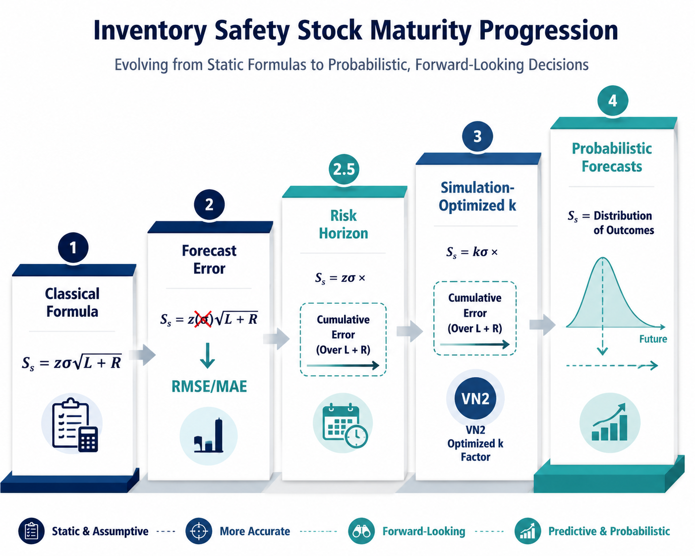
Machine learning does not improve safety stock optimization by sprinkling intelligence over that equation. It changes the calculation by replacing weak assumptions one by one: demand variability becomes forecast error, the square-root risk-horizon shortcut becomes cumulative error measurement, the z-score becomes a simulation-optimized factor, and static historical averages give way to probabilistic forecasts that look forward.

Nicolas Vandeput’s May 2026 four-level maturity framework is a useful way to inspect those substitutions. It should not be treated as an industry standard or a certified ladder every company must climb in order. It is better used as a diagnostic lens: which assumption in the current model is doing the most damage, and what would a more realistic replacement look like? [1]
Start With the Formula, Not the Software
In the classical formula, each term carries a promise. The service factor says how much protection the business wants. Demand standard deviation estimates how much demand moves around. Lead time and review period define the exposure window. Put together, they produce a buffer.
That is also why the formula survives so many planning cycles. Everyone can point to a cell and explain the logic. The spreadsheet has a kind of political advantage: it is auditable, even when it is wrong in ways the audit does not catch.
The machine learning version of the conversation should not begin with a model name. It should begin with the same equation and a sharper question: which input is pretending to measure something it does not actually measure?
| Formula component | Classical assumption | ML-oriented replacement |
|---|---|---|
| σ | Demand variability represents uncertainty | Forecast error measures how wrong the planning signal is |
| √(L+R) | Risk accumulates cleanly under independence assumptions | Cumulative forecast error is measured over the full risk horizon |
| z | Cycle service level maps cleanly to the desired service outcome | Simulation-optimized k factors target the inventory behavior planners care about |
| Historical averages | The past average is a stable guide to the next period | Probabilistic forecasts reflect expected future conditions |
| Lead time input | Supplier delay behaves like a tidy statistical distribution | Supplier reliability signals inform replenishment uncertainty |
The First Upgrade: Replace Demand Variability With Forecast Error
The most common failure is also the easiest to miss. Demand variability and forecast error are not the same thing.
A SKU can have volatile demand and still be forecastable. Think of a seasonal item whose weekly sales rise sharply into peak and then fall away. The demand line moves, but if the pattern is known and the forecast follows it, the planner does not need safety stock for the movement itself. The planner needs protection against the miss.
The opposite can also happen. A slow mover may look calm in historical demand, yet the forecast can still be badly wrong because orders are intermittent, customer timing is lumpy, or the item is managed through sparse signals. In that case, a low σ can produce a false sense of control. The spreadsheet has not found a stable item; it has found a history that hides the actual planning error.
Vandeput’s Level 1 to Level 2 shift replaces demand standard deviation with forecast error measures such as RMSE or MAE. The practical change is simple but important: safety stock is no longer calculated from how much demand moved around; it is calculated from how wrong the forecast tended to be. [1]
That substitution changes the planning conversation. If the buffer is high, the team can ask whether the forecast model is missing promotions, seasonality, customer ordering patterns, or launch effects. If the buffer is low and service misses, the team can inspect whether the error metric is being calculated at the same level where replenishment decisions are made. The safety stock number becomes connected to forecast performance instead of floating beside it.
This is also where many implementations should pause. A company does not need a probabilistic forecasting platform to stop using demand volatility as a proxy for uncertainty. It needs a clean history of forecasts and actuals, a consistent error metric, and enough discipline to calculate error at the item-location-time level where inventory is actually planned.
Why RMSE and MAE Change the Behavior of the Buffer
RMSE and MAE are not interchangeable decorations. RMSE penalizes larger errors more heavily, so it will tend to react harder when the forecast occasionally misses badly. MAE is easier to interpret as an average absolute miss. The maturity shift is toward forecast-error measures, not a universal claim that one metric is always superior.
The operating choice should follow the consequence. If a few large misses create the worst service failures, a metric that responds strongly to large errors may be appropriate. If the team needs a stable and explainable planning measure across many SKUs, a simpler average absolute error may be easier to govern. Either way, the model has moved closer to the actual uncertainty the planner faces.
The Bigger Repair: Stop Trusting √(L+R) When Errors Accumulate
The next weak point is less visible because it looks mathematically respectable. The term √(L+R) expands uncertainty across the lead time plus review period. In many spreadsheets, it is accepted without much discussion because it gives a clean way to scale the buffer as the exposure window grows.
The problem is what the shortcut assumes. It treats the accumulation of uncertainty as if errors behave nicely across the risk horizon. In actual planning, errors can cluster. A forecast can be biased for several periods in a row. A replenishment cycle can span a promotion window. A review cadence can force the planner to live with a bad signal until the next order opportunity. The item does not care that the formula expected errors to diversify cleanly.
Vandeput’s Level 2.5 addresses this by measuring cumulative forecast error over the full risk horizon instead of applying the square-root shortcut. The risk horizon still includes the lead time and review period, but the calculation asks a more operational question: over the full period in which the next replenishment decision cannot rescue us, how wrong can the forecast be? [1]
That sounds like a small change until peak season arrives. A weekly error that seems manageable in isolation can become a service problem when several weeks of under-forecasting stack inside the same replenishment exposure. The classical shortcut may dampen the risk because it is scaling a per-period estimate. Cumulative error measurement looks at the total miss over the decision window.
This is usually the point where the spreadsheet starts to feel less innocent. The formula may be calculating exactly what it was built to calculate, but the business is using the answer for a different question. The planner is not protecting one independent period. The planner is protecting the whole interval between the moment an order decision is made and the moment the next decision can materially correct it.
A Practical Way to Inspect the Risk Horizon
A useful diagnostic is to take a sample of item-location combinations and compare two views side by side. First, calculate the existing safety stock using the current σ and √(L+R) logic. Then calculate historical cumulative forecast error across the same replenishment exposure window. The goal is not to rebuild the whole policy in one workshop. It is to see where the current model is systematically under- or over-reading the exposure.
- Use the same planning grain as the replenishment decision, not a convenient aggregate.
- Include both lead time and review period in the exposure window.
- Measure forecast misses cumulatively across that window.
- Separate under-forecast exposure from over-forecast exposure when service and excess inventory have different consequences.
- Compare the result with actual stockout and excess patterns before changing the policy globally.
For teams already exploring seasonal buffers, this is the natural bridge to more dynamic methods. The adjacent implementation problem is not “AI inventory” in the abstract; it is whether the current exposure-window calculation knows when the future risk is concentrated. A dynamic safety stock approach for seasonal SKUs belongs here, not as a separate planning fashion.
The Service Factor Is Not Sacred
After σ and the risk horizon are repaired, the z-score deserves its own inspection. In the classical setup, z translates a target service level into a safety factor. The calculation is elegant, but the service target it represents is often not the one the business argues about in the S&OP meeting.
Cycle service level and fill rate are different service concepts. Cycle service level concerns the probability of not stocking out during a replenishment cycle. Fill rate concerns the share of demand fulfilled from stock. A policy can look acceptable under one lens and disappoint under the other, especially when order quantities, demand size, and replenishment timing interact.
Vandeput’s Level 3 replaces the theoretical z-score with simulation-optimized k factors. Instead of assuming the service factor maps neatly to the desired operational result, the policy is tested through simulated inventory behavior and the factor is tuned against the service outcome being targeted. [1]
The VN2 inventory competition in 2025 gives this idea some competitive support: the simulation-optimized approach beat 86% of competing policies. That result is meaningful as evidence that simulation-based tuning can perform well in a benchmark setting. It should not be stretched into a universal promise that any company adopting this method will reduce inventory by a fixed amount or achieve a guaranteed ROI. [2]
The operational attraction is clear. A planner can test how a proposed k factor behaves under the actual ordering policy, forecast error pattern, lead time assumptions, and demand profile. The model can show whether a buffer that looks reasonable in formula terms produces too many small stockouts, too much stranded inventory, or an acceptable tradeoff.
This is where broader AI inventory management discussions can become useful, as long as they stay tied to the decision rule. Vendor examples of simulation-driven reorder parameters, including enterprise inventory optimization tools, are relevant when they show how reorder points, order-up-to levels, or safety factors are tuned through scenario testing. They are less useful when they only relabel the same static formula with an AI badge.
Level 4: Forecast the Distribution, Not Just the Average
The Level 4 move is more ambitious: probabilistic distribution forecasts connect safety stock to future conditions rather than relying on static historical averages. In Vandeput’s framework, this is the point where the model can respond to the fact that next month’s uncertainty is not necessarily the average uncertainty from the past. [1]
Seasonality is the cleanest reason this matters. A static historical buffer can flatten peak and trough requirements. It may recommend too little protection before the seasonal climb and too much after the peak has passed. The issue is not that the formula forgot seasonality as a concept; the issue is that the inputs often summarize history in a way that smooths out the period-specific risk the planner is about to face.
A probabilistic forecast gives the safety stock calculation a distribution of possible future demand outcomes. The buffer can then respond to the expected range for the coming period rather than to a backward-looking average. That matters most where forecast uncertainty changes by season, lifecycle stage, promotion timing, or customer mix.
This is also the point where predictive analytics in supply chain planning stops being a dashboard topic and becomes a replenishment input. The forecast is no longer just a number passed to supply planning; it carries uncertainty information the inventory policy can use.
Lead Time Variability Belongs in the Same Conversation
Demand uncertainty usually gets the attention because it is easier to connect to forecasting. Lead time uncertainty can be just as damaging. If a supplier regularly ships late, ships inconsistently, or behaves differently by lane or season, a tidy lead time assumption can make the safety stock policy look more precise than it is.
The machine learning contribution here is not that supplier risk becomes magically knowable. It is that the model can use supplier reliability signals rather than forcing lead time into a neat normal-distribution assumption. Reliability ratings, observed delivery behavior, and replenishment history can inform the uncertainty attached to the inbound side of the equation.
That companion issue matters when planners diagnose service misses. If demand was forecast well but inbound supply arrived late, increasing demand-side safety stock may hide the symptom while leaving the replenishment assumption untouched. The next upgrade may belong in lead time modeling, not in a more sophisticated demand model.
A Maturity Model for the Calculation You Have Now
The table below uses Vandeput’s framework as a practical diagnostic. It is not a certification scheme. It is a way to locate the assumption currently carrying the most risk in the safety stock calculation. [1]
| Maturity level | Current calculation logic | Main assumption | Likely symptom | Next practical upgrade |
|---|---|---|---|---|
| Level 1 | Classical formula: Ss = zσ√(L+R) | Demand variability is a sufficient proxy for uncertainty | Buffers look mathematically correct but miss forecast-driven service problems | Replace demand variability with forecast error |
| Level 2 | Safety stock uses RMSE, MAE, or another forecast-error measure | Per-period forecast error can be scaled through the traditional horizon logic | Peak-season misses or multi-period bias are understated | Measure cumulative forecast error across the full risk horizon |
| Level 2.5 | Safety stock uses cumulative forecast error over lead time plus review period | The service factor still maps well enough to the desired operating outcome | Cycle-service math does not match fill-rate behavior | Use simulation to optimize k factors against the service measure that matters |
| Level 3 | Simulation-optimized k factors replace fixed z-score logic | Historical patterns remain a sufficient guide to future uncertainty | Buffers lag seasonal, lifecycle, or promotion-driven shifts | Move toward probabilistic distribution forecasts |
| Level 4 | Probabilistic forecasts drive period-specific safety stock | Future uncertainty can be estimated directly enough to inform policy | Governance, data quality, and explainability become the limiting factors | Monitor model behavior and upgrade the weakest remaining input, including lead time variability |
Most organizations do not need to jump straight to Level 4. If the spreadsheet still uses demand standard deviation, the highest-return repair may be to connect safety stock to forecast error. If peak exposure is the recurring failure, the risk-horizon calculation deserves attention before the team debates algorithms. If service is judged by fill rate, simulation-optimized factors may matter more than another round of forecast tuning.
That is the practical value of safety stock optimization with machine learning. It does not make the old formula magical. It takes the formula apart, finds the assumption that no longer matches operations, and replaces that part with a better estimate.
References
- Outgrowing the Safety Stock Formula, Medium, May 2026.
- VN2 inventory competition results, 2025.
Comments
Join the discussion with an anonymous comment.