

Why Data Architecture Defines Demand Forecasting Capability
When supply chain technology evaluators shortlist AI demand forecasting platforms, the conversation typically centers on feature checklists: Does it support probabilistic forecasting? Can it handle 100,000 SKUs? What ERP integrations are available? These questions matter, but they obscure a more fundamental differentiator that determines whether a tool will deliver transformative accuracy or merely incremental improvement over spreadsheets.
That differentiator is data architecture. Specifically, whether the platform treats demand as a set of independent time-series (one per SKU-store combination) or as a relational graph where products, promotions, stores, suppliers, and transactions exist as connected nodes. This distinction is not an implementation detail. It is the single largest determinant of forecast quality for any business where demand for one product depends on the availability, pricing, or promotion of another.
The evidence is stark. According to analysis from Kumo.ai, time-series-only demand forecasting models structurally miss 25–30% of demand signal because they forecast each SKU-store pair in isolation. When Product A stocks out and demand shifts to Product B, a time-series model trained only on Product B's history has no mechanism to capture that transfer. The same blind spot applies to promotional lift interactions: a promotion on one product can cannibalize demand for another, but isolated models cannot represent that relationship.
This comparison examines seven leading AI demand forecasting tools through the lens of data architecture. We evaluate how each platform handles cross-product substitution, promotional signal propagation, and multi-table relationships — the capabilities that separate genuinely intelligent forecasting from automated curve-fitting.
The Seven Tools at a Glance: Approach and Positioning
The seven tools in this comparison fall into three broad architectural categories: integrated planning platforms, AutoML platforms, and relational/graph-based platforms. Each category makes distinct trade-offs between planning workflow breadth and depth of demand signal capture.
- o9 Solutions: An integrated planning platform that combines demand, supply, and financial planning in a single data model. o9 uses a graph-based in-memory database to represent product, location, and supplier relationships, enabling multi-echelon inventory optimization (MEIO) and cross-product signal capture. Target buyer: large enterprises with complex multi-echelon supply chains. Implementation timeline: 6–18 months.
- Blue Yonder: A full-suite supply chain planning platform with AI/ML capabilities embedded across demand, inventory, and fulfillment planning. Blue Yonder's Luminate platform uses a unified data model but historically has been stronger on breadth of planning workflows than on native cross-product substitution handling. Target buyer: enterprise retail, CPG, and manufacturing. Implementation timeline: 6–18 months.
- Kinaxis Maestro: A concurrent planning platform that connects demand, supply, and inventory planning in a single environment. Kinaxis uses a patented in-memory engine for what-if scenario analysis but relies on time-series models for core demand forecasting. Target buyer: mid-market to enterprise with complex supply chain networks. Implementation timeline: 6–12 months.
- RELEX: A retail-focused planning platform with strong demand forecasting, replenishment, and space planning capabilities. RELEX uses a unified data model that connects product, store, and promotion data, making it effective for retail substitution and promotional lift capture. Target buyer: retail and CPG companies. Implementation timeline: 3–9 months.
- Anaplan: A connected planning platform that supports demand, supply, and financial planning through a hyperblock calculation engine. Anaplan's demand forecasting module is strong on collaborative planning but relies on user-defined models rather than native AI/ML for cross-product signal capture. Target buyer: enterprise with strong planning maturity. Implementation timeline: 6–12 months.
- DataRobot: An AutoML platform that automates the development and deployment of time-series forecasting models. DataRobot excels at rapid model iteration and handles thousands of SKUs efficiently, but its architecture is fundamentally time-series-based, forecasting each SKU-store pair independently. Target buyer: organizations with data science teams seeking to augment existing forecasting workflows. Implementation timeline: 3–6 months.
- Kumo.ai: A relational AI platform purpose-built for demand forecasting on connected data. Kumo represents products, stores, transactions, promotions, and suppliers as nodes in a graph, enabling native capture of cross-product substitution, promotional lift interactions, and supplier constraint propagation. Target buyer: mid-market to enterprise with complex demand patterns. Implementation timeline: 3–9 months.
For detailed profiles of o9 Solutions, Blue Yonder, and Kinaxis, see the dedicated vendor profile articles on this site.
Structured Comparison: How the Tools Handle Cross-Table Demand Signals
The following matrix compares the seven tools across six evaluation dimensions that directly reflect data architecture capability. These dimensions were selected because they differentiate tools on the ability to capture demand signals that span multiple products, locations, and time periods.
| Tool | Core Approach | Cross-Product Substitution | Multi-Table Native | Promotional Lift | Granularity | Best-Fit Scenario |
|---|---|---|---|---|---|---|
| o9 Solutions | Integrated planning platform with graph-based in-memory DB | Yes — native via graph model | Yes — products, locations, suppliers, promotions in unified model | Yes — captures cross-product cannibalization and halo effects | SKU-store-location with multi-echelon | Large enterprise with complex multi-echelon supply chains |
| Blue Yonder | Full-suite SCP with AI/ML embedded | Partial — via unified data model but limited native substitution | Partial — unified model but historically time-series-based forecasting | Yes — promotion planning module | SKU-store-location | Enterprise retail, CPG, manufacturing |
| Kinaxis Maestro | Concurrent planning with in-memory engine | Limited — time-series models per SKU-location | Partial — concurrent planning connects data but forecasting is per-series | Yes — promotion planning with what-if scenarios | SKU-location with multi-echelon | Mid-market to enterprise with complex networks |
| RELEX | Retail-focused unified planning platform | Yes — native via unified product-store model | Yes — products, stores, promotions in single model | Yes — strong promotion and substitution modeling | SKU-store with space and replenishment | Retail and CPG with high SKU velocity |
| Anaplan | Connected planning with hyperblock engine | Limited — user-defined models, not native AI | Partial — connected planning but forecasting is model-defined | Yes — collaborative planning with manual inputs | SKU-location with user-defined hierarchies | Enterprise with strong planning maturity |
| DataRobot | AutoML time-series platform | No — each SKU-store forecasted independently | No — time-series per entity | No — requires manual feature engineering | SKU-store with automated model selection | Organizations with data science teams augmenting existing workflows |
| Kumo.ai | Relational AI on graph-based data model | Yes — native via graph relationships | Yes — products, stores, transactions, suppliers, promotions as nodes | Yes — captures lift interactions across products and locations | SKU-store with connected signals | Mid-market to enterprise with complex demand patterns |
The Substitution Effect Blind Spot: Why Time-Series Models Miss 25–30% of Demand Signal
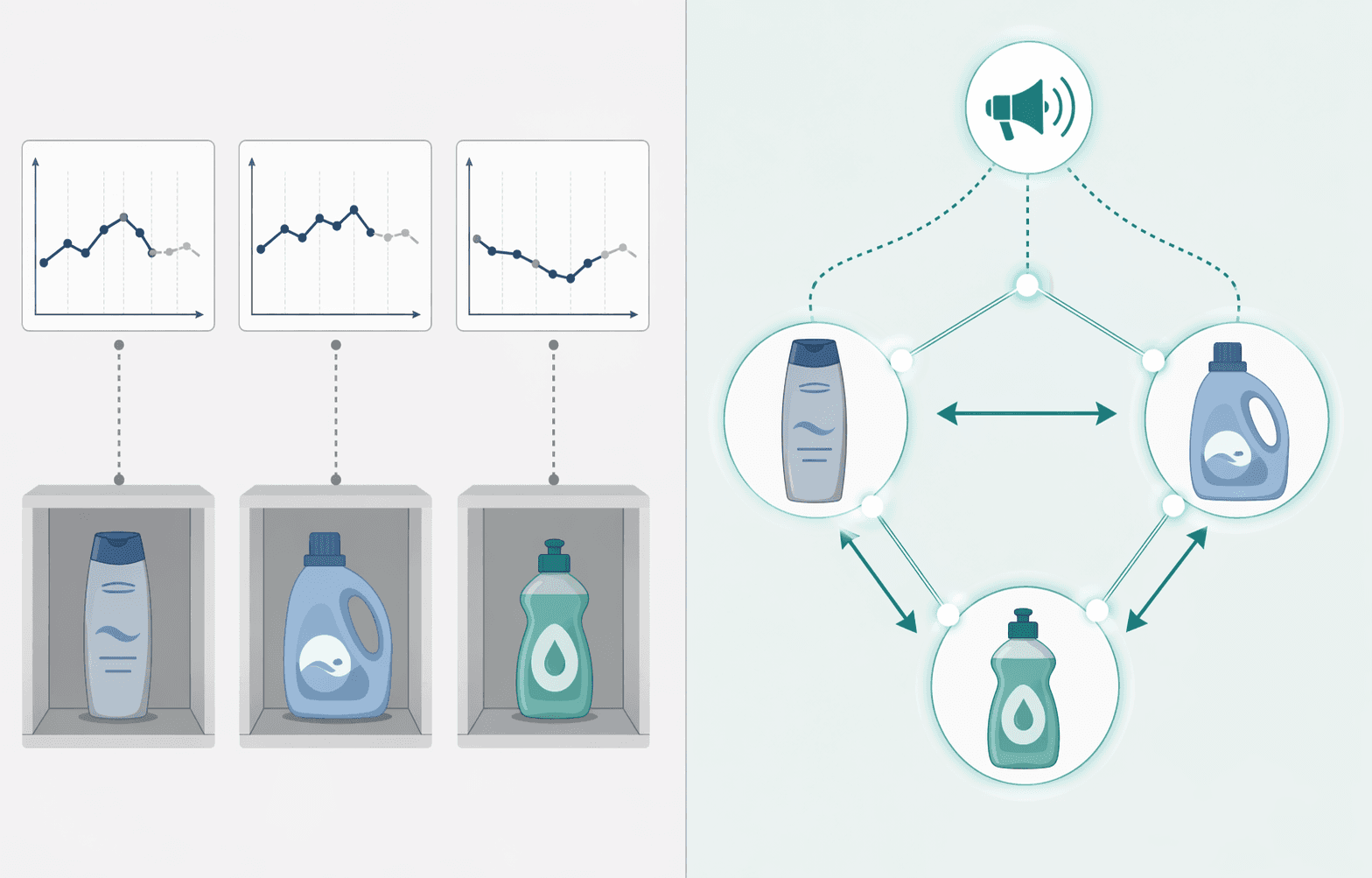
The substitution effect is the most consequential blind spot in time-series-only demand forecasting. When a product stocks out, is promoted, or changes price, demand does not disappear — it shifts to substitute products. A time-series model trained on each SKU-store pair independently has no mechanism to represent this transfer. The result is systematic forecast error that aggregate accuracy metrics mask.
The magnitude of this blind spot is substantial. According to Kumo.ai's analysis, time-series models miss 25–30% of demand signal because they cannot capture cross-product relationships. In retail and CPG environments, promotions drive 20–40% of volume, and cross-product substitution affects 5–8% of SKUs on a weekly basis. For a retailer with 50,000 SKUs, that means 2,500 to 4,000 products are experiencing substitution-driven demand shifts every week — shifts that time-series models cannot represent.
The practical consequence is that a platform reporting 92% aggregate accuracy may perform at 60% accuracy on high-velocity, promotion-sensitive items where replenishment decisions are made. As Invisible Technologies notes in their evaluation framework, a platform that achieves 92% aggregate accuracy but performs at 60% on high-velocity items is not solving the problem — it is averaging over it.
For a deeper treatment of the substitution effect in retail and CPG contexts, see the AI demand forecasting in retail and CPG use-case article. The current comparison uses the substitution effect as a vendor differentiator rather than a standalone concept.
Vendor Selection Decision Matrix by Supply Chain Complexity Profile
The right tool depends on the complexity of your demand patterns, not on the size of your company or the number of SKUs. The following decision matrix maps vendor choice to four supply chain complexity profiles, with implementation timelines and typical ROI benchmarks drawn from enterprise deployments.
| Complexity Profile | Characteristics | Recommended Tools | Implementation Timeline | Typical ROI Benchmarks |
|---|---|---|---|---|
| Simple / Stable | Low SKU count, stable demand, minimal promotions, no substitution effects | DataRobot, traditional time-series models | 3–6 months | 20–50% forecast error reduction (McKinsey 2022); 15–20% cost savings (Capgemini) |
| Promotional / Seasonal with Substitution | Moderate SKU count, frequent promotions, cross-product substitution, seasonal patterns | Kumo.ai (relational AI), RELEX | 3–9 months | 25% overstock reduction; $2–5M working capital freed per quarter (Kumo.ai enterprise benchmarks) |
| Multi-Echelon Enterprise | High SKU count, multiple echelons (plants, DCs, stores), complex supplier networks, global operations | o9 Solutions, Blue Yonder, Kinaxis | 6–18 months | 50% forecast error reduction; 65% fewer lost sales; 50% overstock reduction (McKinsey consumer goods) |
| High-Velocity Retail | Very high SKU count, rapid turnover, space constraints, frequent promotions, strong substitution effects | RELEX, Kumo.ai | 3–9 months | 85% reduction in stockouts and overstocks (OnePint.ai); 3–5% profit margin improvement (Drivepoint) |
Enterprise benchmarks from Kumo.ai show that organizations switching from isolated time-series to relational demand models achieve 25% overstock reduction and free $2–5 million in working capital per quarter. These figures align with broader industry data: McKinsey reports that AI-driven forecasting can reduce supply chain costs by up to 15%, and Deloitte finds that AI cuts working capital by 15%, freeing $200 billion globally. Gartner states that 30% of AI spend in supply chains yields 3x ROI.
For a broader view of the AI supply chain tools landscape beyond demand forecasting, see the AI supply chain tools buyer's comparison.
How to Run a Proof-of-Concept on Your Own Data
A well-designed proof-of-concept (POC) is the most reliable way to determine which tool's data architecture matches your demand complexity. The following approach is structured to surface the architectural differences that matter, rather than comparing feature lists.
- Start with failure-mode analysis, not vendor feature lists. Identify the SKUs and categories where your current forecasting performs worst — typically high-velocity, promotion-sensitive, or seasonal items. These are the cases where data architecture differences will be most visible.
- Ask vendors to run back-cast simulations against a historical slice of your own data. Provide 12–24 months of historical sales data including promotion calendars, pricing changes, and stockout events. Require vendors to forecast a holdout period (the most recent 3–6 months) and report accuracy at the SKU-store level, not just at aggregate category level.
- Test on high-velocity and promotional SKUs specifically. A platform that achieves 92% aggregate accuracy but performs at 60% on high-velocity items is not solving the problem — it is averaging over it. Request separate accuracy reports for your top 20% of SKUs by volume and for items with frequent promotions.
- Evaluate both forecast accuracy and planner trust. A technically accurate model that planners do not trust will not be used. Include planners in the POC evaluation and ask them to review the forecast outputs for face validity. Relational models that show why a forecast changed (e.g., "forecast increased because Product B stocked out") tend to build trust faster than black-box time-series models.
- Measure implementation effort, not just model accuracy. Ask vendors to document the data preparation, integration, and configuration work required. Relational AI platforms typically require 3–9 months, while integrated planning platforms require 6–18 months. The total cost of ownership includes ongoing model maintenance, retraining, and governance.
Key Takeaways and Next Steps for Evaluators
The data architecture divide — time-series vs. relational — is the single most important factor in determining whether an AI demand forecasting tool will deliver transformative accuracy or marginal improvement. For organizations where demand for one product depends on the availability, pricing, or promotion of another, time-series-only tools structurally miss 25–30% of demand signal.
- Match data architecture to demand complexity. If your business has substitution effects, promotional lift interactions, or supplier constraints that propagate across products, prioritize tools with relational or graph-based architectures (Kumo.ai, o9 Solutions, RELEX). If your demand is stable and independent, time-series AutoML platforms (DataRobot) may be sufficient.
- Prioritize tools that natively capture cross-product and promotional signals. Integrated planning platforms (o9, Blue Yonder, Kinaxis) offer breadth of planning workflows but vary in their native ability to capture cross-product substitution. Relational AI platforms (Kumo.ai) and retail-focused platforms (RELEX) are stronger on signal depth.
- Budget for 3–18 months of implementation depending on platform breadth. Relational AI platforms typically require 3–9 months; integrated planning platforms require 6–18 months. The longer timeline for integrated platforms reflects data integration, model configuration, and organizational change management, not just software deployment.
- Run a structured POC on your own data before making a decision. Focus on failure modes, test on high-velocity and promotional SKUs, and evaluate both forecast accuracy and planner trust. Request back-cast simulations rather than forward-looking demonstrations.
- Consult the individual vendor profiles for deeper dives: o9 Solutions, Blue Yonder, and Kinaxis provide detailed capability assessments beyond the scope of this comparison.
The AI demand forecasting software market is projected to grow from $827.7 million in 2025 to $2,070.1 million by 2035 (LatentView). As the market expands, the gap between tools that merely automate curve-fitting and tools that truly understand demand relationships will widen. Organizations that invest in the right data architecture today will have a compounding advantage in forecast accuracy, inventory efficiency, and working capital performance.
Comments
Join the discussion with an anonymous comment.