Why Retail and CPG Forecasting Is Harder Than It Looks
Retail and consumer packaged goods (CPG) supply chains operate at a level of granularity that most forecasting systems were never designed to handle. A national grocery chain might manage 50,000 SKUs across 2,000 store locations, each with its own local demand pattern, promotional calendar, and shelf-space allocation. Multiply those dimensions by 52 weeks, and the number of individual forecasts required per year runs into the billions.
Three structural forces compound this complexity. First, SKU proliferation has accelerated faster than most planning systems can absorb. Retailers now carry more variants, sizes, and flavors than ever, each with a shorter lifecycle and thinner sales history. Second, multi-channel fragmentation means the same SKU flows through physical stores, e-commerce fulfillment centers, and direct-to-consumer channels, each with different demand signals and lead times. Third, short product lifecycles — particularly in fashion, seasonal CPG, and private-label goods — leave planners with sparse historical data to train models on.

The practical consequence is that a forecast that works at the category or region level often collapses when pushed down to the SKU-store-week level. A model that predicts 12,000 units of laundry detergent for the Northeast region may be off by 40% or more when asked to allocate those units across individual stores in Boston, Portland, and Scranton — each with different brand preferences, price sensitivities, and competitive landscapes.
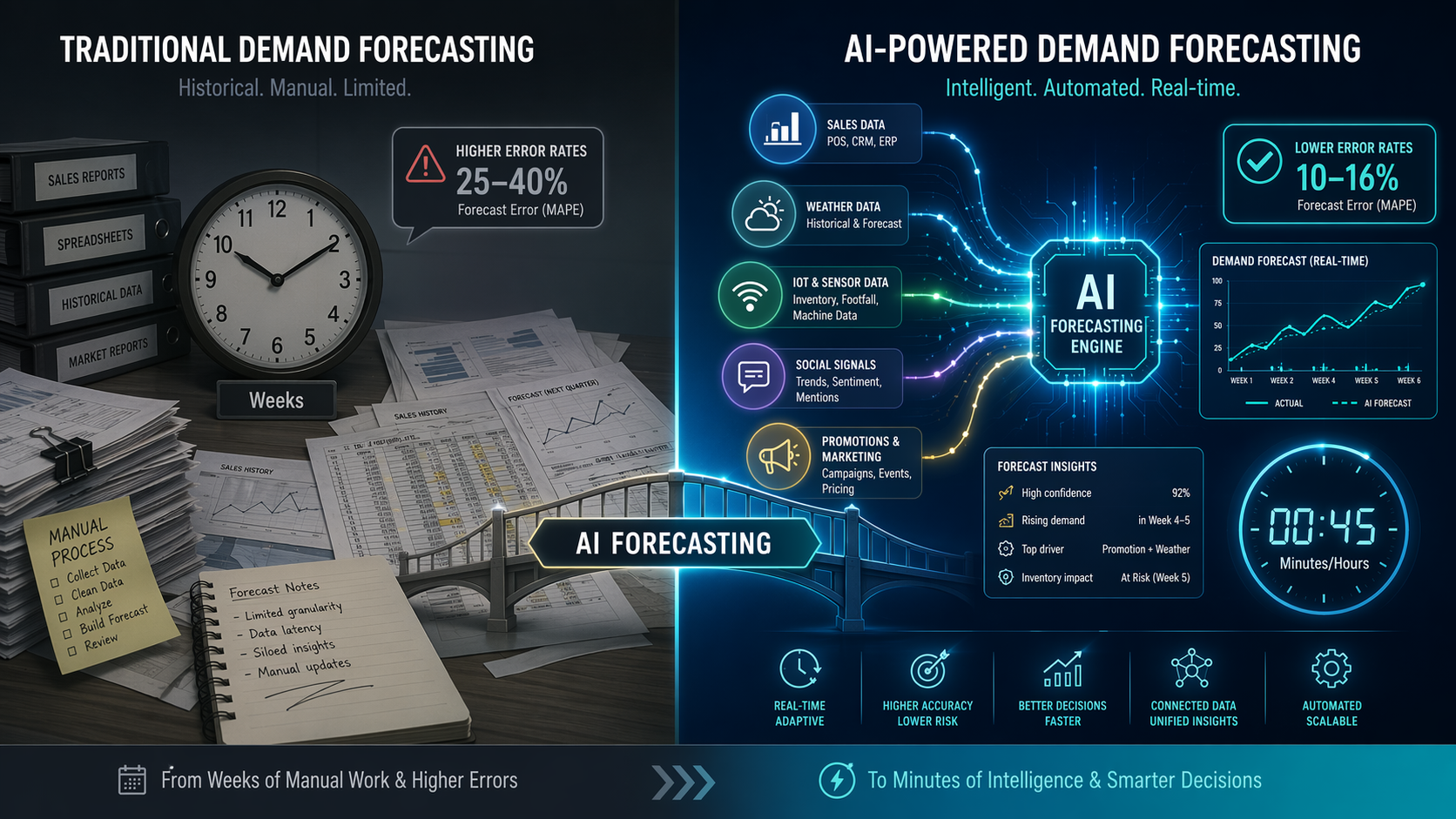
This is not a problem that can be solved by throwing more data at a time-series model. The structural challenges of retail and CPG demand — cross-product substitution, promotional lift interactions, and supplier constraint propagation — are fundamentally relational. They involve connections between SKUs, stores, promotions, and suppliers that isolated time-series models cannot see.
The Three Blind Spots of Time-Series Models in Retail
Time-series models — whether classical (ARIMA, exponential smoothing) or machine learning-based (Prophet, XGBoost) — share a fundamental limitation: they treat each SKU-store pair as an independent forecasting problem. The model looks at the historical sales of SKU A in Store 1 and projects that pattern forward. It has no mechanism to know that SKU B, sitting on the adjacent shelf, is a near-perfect substitute, or that a 20% discount on SKU C in urban stores will cannibalize SKU D in suburban stores.
This structural blind spot manifests in three specific ways that are particularly damaging in retail and CPG environments.
1. Cross-Product Substitution: The Invisible Demand Shift
When a shopper walks into a store and finds their preferred brand of yogurt out of stock, they do not simply leave. They pick up a competing brand, a different flavor, or a larger size. That demand shift — from the out-of-stock SKU to a substitute — is invisible to a time-series model trained only on the historical sales of each individual SKU.
According to benchmarks from Kumo.ai, cross-product substitution affects 5–8% of SKUs weekly in retail and CPG environments and is the largest source of forecast error after basic seasonality. A model that cannot see substitution will systematically under-forecast the substitute SKU during stockout events and over-forecast the primary SKU when it returns to stock.
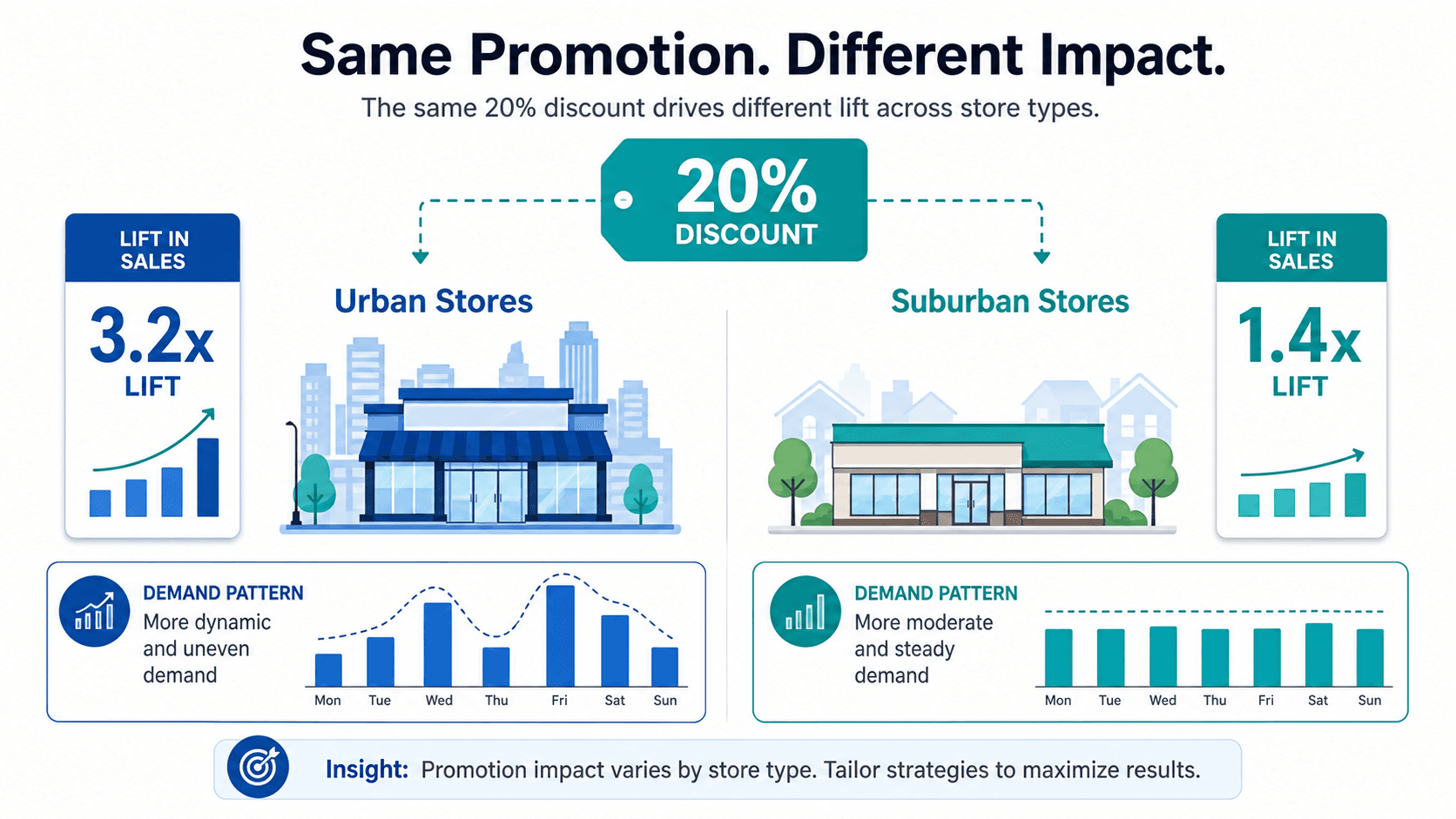
2. Promotional Lift Interactions: The Same Deal, Different Results
Promotions drive 20–40% of volume in CPG categories, making them the single largest demand lever available to retailers and manufacturers. Yet most forecasting models treat promotional lift as a simple binary flag: if a promotion is active, apply a fixed multiplier to the baseline forecast.
This approach fails because promotional lift is not uniform. A 20% discount on a premium SKU in an urban store cluster might produce a 3.2x lift, while the same discount on the same SKU in a suburban store cluster produces only a 1.4x lift, per Kumo.ai benchmarks. The difference is driven by store-level demographics, competitive density, and the product's price elasticity — variables that a time-series model cannot incorporate as interaction effects.
3. Supplier Constraint Propagation: The Ripple Effect
When a supplier experiences a production delay or raw material shortage, the impact does not stop at that supplier's direct shipments. It propagates across the entire product portfolio. A delay in packaging materials might affect 50 SKUs simultaneously. A shortage of a key ingredient might force reformulations or substitutions across multiple product lines.
Time-series models have no mechanism to represent these dependencies. Each SKU's forecast is generated independently, so the model cannot learn that a constraint on Supplier X should reduce the forecast for all SKUs that depend on that supplier. The result is systematic over-forecasting during supply disruptions and missed revenue opportunities when constraints ease.
How Relational AI (Graph Neural Networks) Captures Cross-Table Signals
Relational AI — specifically graph neural networks (GNNs) — addresses these blind spots by changing the fundamental data structure used for forecasting. Instead of treating each SKU-store pair as an independent time series, a graph-based model represents SKUs, stores, promotions, and suppliers as interconnected nodes in a graph. Edges between nodes encode relationships: substitution affinity between SKUs, promotional eligibility between a promotion and a store cluster, supply dependency between a supplier and its SKUs.
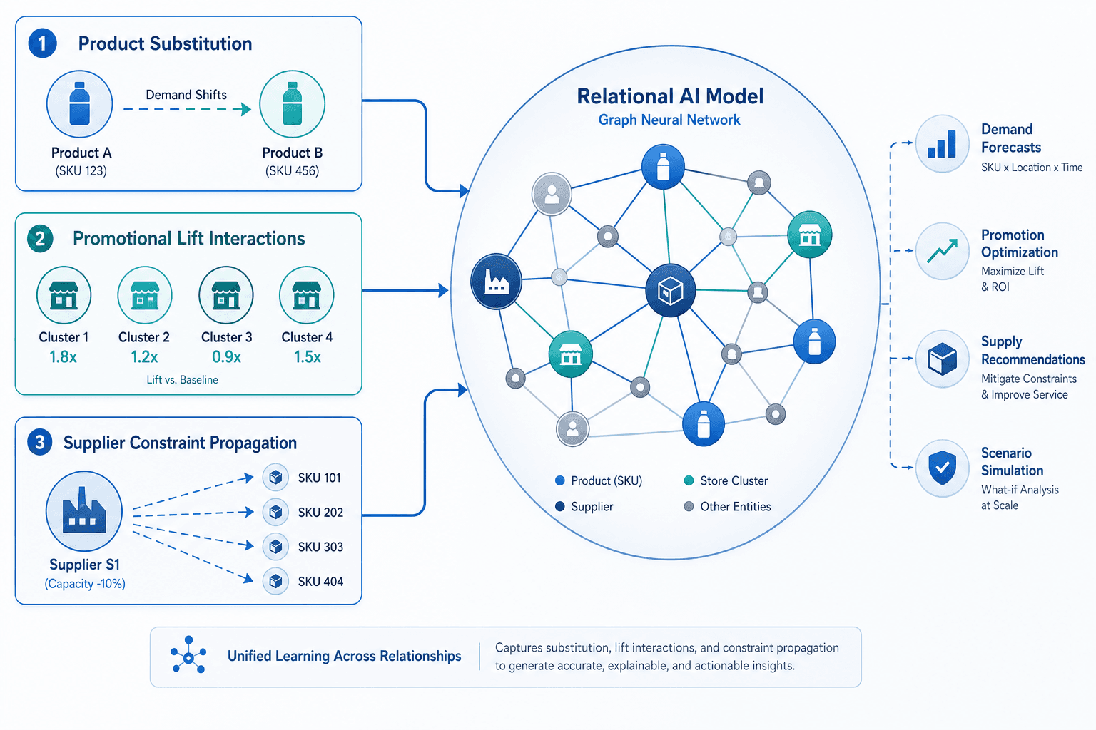
When the model generates a forecast for a specific SKU-store pair, it does not only look at that pair's historical sales. It aggregates information from neighboring nodes in the graph: the sales of substitute SKUs in the same store, the promotional calendar for that store cluster, the current lead time from the supplier. This message-passing architecture allows the model to learn complex interaction effects that are invisible to isolated time-series models.
The impact on forecast accuracy is substantial. On the SAP SALT enterprise benchmark, Kumo.ai's relational forecasting model (KumoRFM) achieved 89% accuracy compared to 75% for PhD data scientists using XGBoost and 63% for LLM+AutoML approaches. More broadly, enterprise benchmarks suggest that relational AI achieves 85–95% SKU-store-week accuracy versus 60–75% for time-series models on the same data.
Companies that have made the switch from isolated time-series to relational demand models report operational improvements beyond accuracy. Kumo.ai benchmarks indicate a 25% reduction in overstock and $2–5 million in freed working capital per quarter. These outcomes reflect the fact that a model which understands substitution and promotional interactions can make more precise inventory allocation decisions — reducing safety stock without increasing stockout risk.
Real Retail Examples: Substitution, Lift, and Constraint Effects in Action
The theoretical advantages of relational AI become concrete when mapped to real retail scenarios. The following table summarizes three common situations where time-series models fail and relational models succeed.
| Scenario | Time-Series Model Behavior | Relational AI Behavior | Business Impact |
|---|---|---|---|
| Stockout on Brand A yogurt shifts demand to Brand B | Forecasts Brand B at baseline; misses 30–50% of actual demand during stockout | Learns substitution affinity from graph; adjusts Brand B forecast upward when Brand A stockout is detected | Reduces lost sales by capturing demand shift; prevents over-ordering when Brand A returns |
| 20% discount on premium SKU in urban vs. suburban stores | Applies same lift multiplier (e.g., 1.8x) to all stores | Learns store-cluster-specific lift: 3.2x in urban, 1.4x in suburban | Optimizes inventory allocation; prevents stockouts in high-lift stores and overstocks in low-lift stores |
| Supplier packaging delay affects 50 SKUs simultaneously | Each SKU forecasted independently; no constraint signal | Supplier node propagates delay signal to all dependent SKUs; forecasts adjusted downward | Prevents $2–5M in excess inventory per quarter (per Kumo.ai benchmarks) |
The substitution example is particularly instructive. In a typical grocery store, 5–8% of SKUs experience a stockout in any given week. For each of those SKUs, demand does not disappear — it shifts to substitutes. A time-series model that cannot see this shift will generate forecasts that are systematically wrong for both the out-of-stock SKU (over-forecast) and the substitute SKU (under-forecast). Over a quarter, these errors compound into significant inventory misallocation.
Promotional Lift Modeling: The Single Largest Demand Driver
Promotions are not just a demand driver — they are the dominant demand driver in CPG, accounting for 20–40% of category volume. Getting promotional lift wrong means getting the entire forecast wrong. Yet most forecasting systems treat promotional lift as a static parameter: a fixed percentage uplift applied whenever a promotion is active.
The reality is far more complex. Promotional lift varies across at least three dimensions:
- Product tier: Premium SKUs tend to have higher price elasticity and thus higher promotional lift than value-tier SKUs.
- Store cluster: Urban stores with higher foot traffic and more competitive density see different lift patterns than suburban or rural stores.
- Promotion type: A percentage discount, a buy-one-get-one offer, and a loyalty-point multiplier each produce different lift profiles, even on the same SKU.
A relational model captures these interactions natively. The graph structure allows the model to learn that a 20% discount on a premium SKU in an urban store cluster produces 3.2x lift, while the same discount on the same SKU in a suburban cluster produces only 1.4x lift. This is not a parameter that a planner sets manually — it is a pattern that the model learns from the data, provided the data includes store-cluster attributes and promotion-type identifiers.
The practical implication is significant. A retailer running a national promotion on a premium SKU might allocate inventory evenly across all stores based on a single lift multiplier. The result: stockouts in high-lift urban stores and excess inventory in low-lift suburban stores. A relational model that captures store-cluster-specific lift enables precise allocation, reducing both lost sales and markdown risk.
Vendor Approaches That Address Retail Complexity
Several vendors have built platforms that address the structural challenges of retail and CPG forecasting, though their approaches differ in methodology, granularity, and integration requirements. The following table summarizes how four representative vendors handle the three blind spots.
| Vendor | Core Methodology | Substitution Handling | Promotional Lift Modeling | Supplier Constraint Handling | Granularity |
|---|---|---|---|---|---|
| Blue Yonder | ML ensemble with proprietary promotion engine | Rule-based substitution detection with manual override | Store-cluster-specific lift curves; promotion interaction effects | Supply constraint propagation via network model | SKU-store-week |
| RELEX | ML with shelf-aware demand sensing | Substitution modeled via product affinity scoring | Promotion × store × product interaction model | Constraint propagation via supply chain network graph | SKU-store-day |
| Kumo.ai | Graph neural network (relational AI) | Native graph-based substitution learning | Graph-based product × store × promotion interaction learning | Native graph-based constraint propagation | SKU-store-week |
| o9 | ML with demand sensing and scenario modeling | Substitution modeled via product attribute similarity | Promotion lift modeled with scenario simulation | Constraint propagation via digital twin | SKU-store-week |
The key differentiator among these vendors is how they handle the relational structure of retail demand. Blue Yonder and RELEX use rule-based or scoring-based approaches to model substitution and promotional interactions, which require manual configuration and ongoing maintenance. Kumo.ai uses a graph neural network that learns these relationships automatically from the data. o9 uses a digital twin approach that allows scenario simulation but requires significant data integration effort.
For demand planning managers evaluating these platforms, the critical question is not which vendor has the highest accuracy on a benchmark, but which vendor's approach aligns with their organization's data maturity, SKU complexity, and integration landscape. A graph-native approach may be overkill for a retailer with 500 SKUs and simple promotion calendars, but essential for a national CPG manufacturer managing 50,000 SKUs across 10,000 stores with complex promotion calendars.
Implementation Considerations for Retail and CPG
Deploying AI demand forecasting at the SKU-store level in retail and CPG environments presents practical challenges that go beyond model selection. These challenges are specific to the structural complexity of retail and CPG — not generic implementation pitfalls.
SKU Volume Scalability
The scale of retail and CPG forecasting is enormous. Amazon uses AI-driven demand forecasting for more than 400 million products, according to Intellias. While most retailers operate at a smaller scale, the principle holds: the forecasting system must handle millions of SKU-store-week combinations without degrading performance. Graph-based models scale differently than time-series models — the computational cost grows with the number of edges (relationships) rather than the number of nodes (SKU-store pairs). Organizations should benchmark their specific SKU-store graph size against vendor scalability claims before committing to a platform.
Data Integration with POS and ERP Systems
Relational AI models require data that many retailers do not currently capture in a structured, accessible format. Substitution patterns require point-of-sale (POS) data at the transaction level, not just aggregated sales. Promotional lift modeling requires promotion calendars with store-cluster assignment, not just national promotion flags. Supplier constraint propagation requires real-time or near-real-time supplier lead time data.
For organizations that lack this data, the first implementation step is not model deployment — it is data infrastructure investment. POS data must be centralized, promotion calendars must be digitized with store-level granularity, and supplier data must be integrated through a supply chain control tower or similar platform.
Model Retraining Cadence
Retail and CPG demand patterns shift rapidly. New product introductions, competitor actions, and changing consumer preferences mean that a model trained on last year's data may be significantly less accurate this year. Graph-based models require retraining when the graph structure changes — when new SKUs are added, stores are opened or closed, or supplier relationships change. Organizations should plan for weekly or bi-weekly retraining cycles during peak seasons and monthly retraining during stable periods.
Staged Adoption Model
The GroupBWT staged adoption model provides a useful framework for retail and CPG organizations:
- Pilot (0–3 months, $100K–$500K): Select a single category or store cluster. Focus on proving that relational AI captures substitution and promotional lift effects that the current system misses. Measure forecast accuracy improvement and inventory reduction.
- Expansion (6–12 months): Scale to multiple categories and store clusters. Integrate supplier constraint data. Begin using relational forecasts for inventory allocation decisions.
- Enterprise (18–24 months): Full deployment across all SKUs and stores. Integrate with S&OP and IBP processes. Use relational forecasts for promotional planning and supplier collaboration.
- Adaptive (36+ months, budgets exceeding $10M): Continuous model retraining with real-time data feeds. Autonomous inventory replenishment decisions for select categories. Full digital twin integration.
For demand planning managers and retail/CPG supply chain practitioners, the path forward is clear: the structural challenges of SKU-store-level forecasting — substitution, promotional lift interactions, and supplier constraint propagation — cannot be solved by incremental improvements to time-series models. They require a fundamentally different approach to representing and learning from the relational structure of retail demand. Graph-based AI offers that approach, with documented accuracy improvements and operational outcomes that justify the investment in data infrastructure and organizational change.
Comments
Join the discussion with an anonymous comment.